Backpropagation
The chain rule that trains neural networks — every gradient in one backward pass
This is where the section comes together. Gradient descent needs the gradient of the cost with respect to every weight; in a network with millions of them, computing those gradients is the hard part, and backpropagation is how it is done. It is nothing more exotic than the chain rule from calculus, applied with ruthless efficiency: run the network forward to get the loss, then walk backward through it once, multiplying local derivatives, and out fall the gradients for every weight at once. That single idea — reverse-mode differentiation — is what makes training deep networks feasible, and it is the engine underneath essentially all of modern machine learning.
The equation
Backpropagation computes \partial L/\partial W by propagating an error signal \delta backward through the layers. At the output layer L and each hidden layer l:
\delta^{(L)} = \nabla_a L \odot f'(z^{(L)}), \qquad \delta^{(l)} = \big(W^{(l+1)\top}\delta^{(l+1)}\big) \odot f'(z^{(l)})
and the gradient for each weight matrix is
\frac{\partial L}{\partial W^{(l)}} = \delta^{(l)}\,\big(a^{(l-1)}\big)^{\top}.
\delta is the loss’s sensitivity to a layer’s pre-activation; \odot is the elementwise product; f' is the activation’s derivative.
What each symbol means
| Symbol | Meaning |
|---|---|
| L | the loss (cost) being differentiated |
| W^{(l)} | weight matrix of layer l |
| z^{(l)} | pre-activations (Wa + b) of layer l |
| a^{(l)} | activations, a = f(z) |
| f'(z) | derivative of the activation |
| \delta^{(l)} | the error signal at layer l, \partial L/\partial z^{(l)} |
| \odot | elementwise (Hadamard) product |
Plain-English explanation
Training a network means nudging each weight in the direction that lowers the loss, and to do that you need to know how sensitive the loss is to each weight — its gradient. A network is a deep composition of functions (weights, then an activation, then more weights, then another activation…), and the chain rule says the derivative through a composition is the product of the derivatives of its pieces. Backpropagation is the bookkeeping that computes that product efficiently. First a forward pass sends the input through the network, recording each layer’s activations and ending in the loss. Then a backward pass starts from the loss and moves layer by layer toward the input, carrying an “error signal” \delta that says how much each layer’s output was to blame; at every weight, the gradient is that error signal times the input the weight saw.
The reason it matters is efficiency. You could estimate each gradient numerically — nudge a weight, see how the loss changes — but that costs a full forward pass per weight, hopeless for a model with millions or billions of them. Backpropagation gets every gradient in a single backward pass, the same cost as one forward pass, because it reuses the error signals it has already computed rather than starting over for each weight. That is the whole reason deep learning is computationally possible. Modern frameworks call the general version automatic differentiation, but it is backprop: build the computation, then differentiate it in reverse.
Why it matters in markets
Backpropagation is the capstone of this section because it is where every other piece plugs in. It differentiates the cost function you chose (MSE or cross-entropy), through the activations you used (sigmoid, softmax, ReLU), to produce the gradients that gradient descent then steps along — and regularisation rides in the same objective to keep the result from overfitting. The neat cancellations you met earlier are backprop’s opening move: pair softmax with cross-entropy and the output error signal is simply \delta = p - y, predicted minus actual, which is why that combination is universal. Backprop is also where the sigmoid’s flaw turns fatal — its derivative peaks at 0.25, so stacking many sigmoids multiplies many sub-quarter numbers together and the error signal vanishes before it reaches the early layers. That vanishing gradient, seen through backprop, is why deep networks switched to ReLU and added normalisation and residual connections.
For markets, backprop is the reason a neural network can, in principle, learn any pattern in the data — and the honest test of whether there is a pattern to learn. The figure trains a small net by backprop to predict the Nasdaq’s next-day direction from its last 20 returns. Backprop does its job flawlessly: the training loss falls steadily as it fits the data. But the validation loss climbs the whole way, and the test accuracy lands at 50% — below the 56% you’d get by always guessing “up.” The network didn’t fail to train; it trained perfectly, and all it learned was the training set’s noise. The most flexible model in this library, driven by its most powerful algorithm, returns the same verdict as the simplest: there is no reliable signal in yesterday’s returns.
A simple worked example
Take the smallest possible network: one input x = 1, one hidden unit with a sigmoid, one linear output, and a target y = 0. With weights w_1 = 0.5 and w_2 = 0.8, the forward pass is z_1 = w_1 x = 0.5, h = \sigma(0.5) = 0.62, \hat y = w_2 h = 0.50, and squared-error loss L = \tfrac{1}{2}\hat y^2 = 0.12. Now backward. The loss’s sensitivity to the output is \partial L/\partial \hat y = \hat y - y = 0.50. Push it through w_2: \partial L/\partial w_2 = (\partial L/\partial \hat y)\cdot h = 0.50 \times 0.62 = 0.31. Keep going into the hidden unit: \partial L/\partial h = (\partial L/\partial \hat y)\cdot w_2 = 0.40, then through the sigmoid’s derivative \sigma'(0.5) = 0.62 \times 0.38 = 0.24, giving \partial L/\partial z_1 = 0.40 \times 0.24 = 0.094, and finally \partial L/\partial w_1 = (\partial L/\partial z_1)\cdot x = 0.094. Each gradient is a running product of local derivatives, and every one reuses the number computed the step before — the chain rule, bookkept backward. (Nudging each weight numerically confirms 0.31 and 0.094 exactly.)
Python implementation
import numpy as np
# backprop by hand for a 1-hidden-layer net:
def forward(x, W1, W2):
    z1 = x @ W1; a1 = 1/(1+np.exp(-z1))      # hidden (sigmoid)
    z2 = a1 @ W2                              # output
    return z1, a1, z2

z1, a1, z2 = forward(x, W1, W2)
delta2 = (z2 - y)                            # output error (MSE)  -> dL/dz2
dW2    = a1.T @ delta2
delta1 = (delta2 @ W2.T) * (a1 * (1 - a1))   # backprop through sigmoid: σ' = a1(1-a1)
dW1    = x.T @ delta1
# then: W -= lr * dW   (that step is gradient descent)
In practice you never write this: loss.backward() in PyTorch runs reverse-mode autodiff — the same algorithm — over an arbitrary computation graph.
Manual / Excel calculation
Backprop is followable by hand on a tiny network exactly as the worked example shows: build a forward column (each cell a function of the last), then a backward column of derivatives multiplied cell by cell (=next_delta * local_derivative). A spreadsheet can even train a 2–3-weight net this way, one row per update — a teaching exercise, not a tool; real networks need the vectorised, autodiff version.
Financial-market example — Nasdaq 100
The figure’s right panel is a 32-unit neural network trained by backpropagation to classify the Nasdaq’s next day as up or down from its previous 20 returns, on a 70/30 time split. Watch the two curves diverge. The training log loss falls from 0.70 toward 0.54 — backprop is working, steadily reshaping thousands of weights to fit the data. The validation log loss does the opposite: it climbs past 1.1, and out-of-sample accuracy comes in at 50%, worse than the 56% base rate of always guessing up.
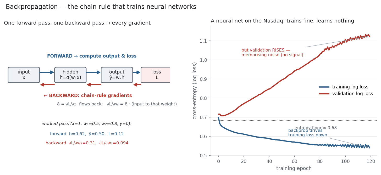
This is the library’s closing note, and a fitting one. Backpropagation is the most powerful optimiser here, wired to the most flexible model here, and it fails exactly the way entropy, cross-entropy, the AR model and the Hurst exponent each said it would — not by failing to optimise, but by optimising perfectly and finding nothing but noise. The training loss dropping is backprop doing its job; the validation loss rising is the market keeping its secret. Everything in this section, from a single mean to a neural network, converges on the same humbling result: the daily direction of a near-efficient index is very close to unpredictable, and the real skill is a model honest enough to admit it.
Same multi_daily.csv as the previous entries (yfinance, adjusted closes). The market panel is a scikit-learn MLPClassifier (32 hidden units) trained by backprop on 20 standardised lagged NDX returns, 70/30 time split; the worked-pass gradients were checked against numerical differentiation. Every number was verified.
Common mistakes
- Confusing backprop with gradient descent. Backprop computes the gradients; gradient descent uses them to update weights — separate steps of one training loop.
- Forgetting the forward-pass caches. The backward pass needs each layer’s activations; store them on the way forward.
- Ignoring vanishing/exploding gradients. Deep stacks of saturating activations multiply small derivatives toward zero; use ReLU, normalisation, or residual connections.
- Hand-deriving gradients in production. Autodiff (PyTorch/TensorFlow) is exact and automatic; manual gradients are for learning.
- Reading a falling training loss as success. As the Nasdaq figure shows, training loss falls even with no signal; judge on validation.
- Thinking a bigger network finds signal that isn’t there. More capacity fits more training noise, not more truth; regularisation and honest validation matter more than depth.