Embeddings

Turning discrete symbols into learned geometry, where nearness means similarity

An embedding maps discrete entities — words, tickers, categories — to dense learned vectors whose geometry encodes similarity, replacing sparse one-hot encoding. The lookup matrix, learning by factorization, and a real asset embedding from Nasdaq co-movement.

The final piece of the deep-learning section closes a loop the others left open. Attention, transformers, every neural network here operates on vectors — but the raw inputs of the world are discrete symbols: words, tickers, sectors, user IDs. Embeddings are the bridge. An embedding maps each discrete entity to a dense, low-dimensional, learned vector, arranged so that geometry encodes meaning — related entities land close together. Where one-hot encoding treats every symbol as an isolated, equidistant token, an embedding discovers and stores the similarity structure among them. It is the input layer of essentially every language model, and, as it happens, a genuinely useful tool for representing the categorical entities of markets.

1. What problem does it solve?

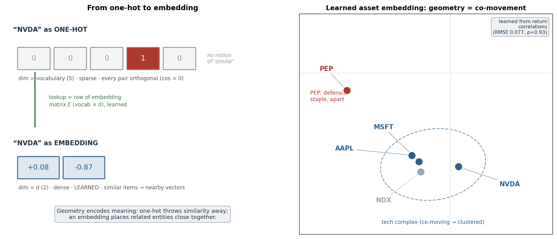
Two problems at once. First, representation: a model needs numbers, but a ticker or a word is a symbol, and the naive fix — a one-hot vector with a 1 in the entity’s slot and 0 elsewhere — is enormous (as long as the vocabulary), sparse, and, crucially, similarity-blind: every pair of distinct one-hot vectors is orthogonal, so “NVDA” is exactly as far from “MSFT” as it is from “PEP”. Second, similarity learning: an embedding replaces that with a short dense vector per entity, learned so that similar entities sit nearby — turning a bag of unrelated symbols into a continuous space where distance and direction mean something.

2. What assumptions does it make?

That the entities have a meaningful similarity structure, and that it can be captured by proximity in a low-dimensional continuous space. The engine behind most embeddings is the distributional hypothesis — “you shall know a word by the company it keeps” — the assumption that entities appearing in similar contexts are similar, so co-occurrence statistics reveal meaning. And it assumes a fixed dimension d is enough to hold the relevant structure.

3. What data does it need?

Many entities together with context or co-occurrence data: large text corpora for word embeddings, return or transaction histories for asset embeddings, interaction logs for user/item embeddings. The richer the co-occurrence signal, the better the geometry. The corollary is a real limitation — rare entities (a thinly traded name, a word seen twice) get poor embeddings, and brand-new entities get none at all until retrained (the cold-start problem).

4. How does it work?

Mechanically an embedding is a lookup table: an embedding matrix E of shape (\text{vocabulary} \times d), where entity i’s vector is simply row i — equivalently, one_hot(i) @ E. The whole content is in how those rows are learned, and there are two routes. End-to-end: make E a layer of a network and train it by backpropagation on a downstream task — the rows become whatever representation best serves the objective. Self-supervised: learn from co-occurrence alone, as in word2vec, which predicts a word’s context and, it turns out, implicitly factorises a co-occurrence matrix — embeddings whose dot products reproduce how often entities appear together. The result is geometry that encodes similarity (cosine distance for relatedness) and even linear analogies (the famous \text{king} - \text{man} + \text{woman} \approx \text{queen}).

That factorisation view makes for a clean, real market demonstration. I learned a 2-dimensional embedding of five Nasdaq names directly from their return correlation matrix, fitting vectors whose dot products reproduce the correlations. The embedding reconstructs the correlation matrix to an RMSE of 0.077 and recovers the similarity ordering almost perfectly (rank correlation 0.93) — and the geometry is exactly what a portfolio manager would draw: the co-moving tech complex (the index, AAPL, MSFT, NVDA) clusters together, while the defensive consumer staple PEP sits well apart, its average similarity to the tech names just 0.39 against 0.95 within the cluster. This is genuine embedding learning — matrix factorisation is precisely what word2vec does under the hood — and it connects straight back to PCA: both are low-rank factorisations of a covariance-like matrix, one for compression, one for placing entities in a similarity space.

Left: one-hot versus embedding. “NVDA” as a one-hot vector is 5-dimensional, sparse, and orthogonal to every other ticker (no notion of similarity); as an embedding it is a short dense vector — a learned row of the embedding matrix — and similar tickers get nearby vectors. Right: a real 2-D asset embedding learned from Nasdaq return correlations. The co-moving tech names cluster; the defensive staple PEP sits apart. Geometry encodes co-movement (reconstruction RMSE 0.077, similarity-ordering ρ = 0.93).

5. What are its strengths?

• Dense and compact. A short vector replaces a vocabulary-length sparse one — far less memory and a far better input to any model.
• Captures similarity. Geometry encodes meaning: nearby vectors are related, so distance and direction are informative.
• Learned, not hand-crafted. The structure comes from data, either task-specific or self-supervised from co-occurrence.
• Transferable. Pretrained embeddings (word2vec, GloVe, and modern contextual ones) carry knowledge into new tasks with little data.
• Enables similarity search, clustering, analogies. A continuous space makes “find the most similar” and “group these” trivial.

6. What are its weaknesses?

• Data-hungry, poor on rare entities. Little co-occurrence signal means a bad vector; new entities have none (cold start).
• Classically static. Plain word2vec gives one vector per word regardless of context — fixed only by contextual embeddings (BERT and later).
• Inherits biases. An embedding faithfully encodes whatever associations — including unwanted ones — are in the training data.
• Opaque dimensions. The axes aren’t individually interpretable, and d is a hyperparameter to tune.
• A representation, not a prediction. It organises entities; it does not, by itself, forecast anything.

7. How could it apply to markets?

This is one of the genuinely useful ideas in the section for quant work, because it captures structure that is there. Embed the categorical entities of markets — tickers, sectors, regimes, exchanges — into a space where geometry means economic similarity, exactly as the figure does: the embedding learned the cross-section’s co-movement and placed peers together. The uses are concrete. Peer and similarity analysis: find the names most “like” a target for hedging, pairs trading, or relative value. Diversification: cluster in embedding space to build baskets of genuinely different exposures. Categorical features: feed a learned embedding of sector or regime into a model instead of a one-hot column, letting related categories share statistical strength. And text: embed news or filings tied to a ticker for sentiment or event detection — the input to your own research pipeline.

The honest boundary is the same one this site keeps drawing, but here it is a boundary, not a disappointment. An embedding represents and organises — it captures the real similarity structure of the cross-section — and it does not predict the daily direction of any single name, which remains the market’s secret. Turning discrete market entities into learnable geometry is real value; expecting that geometry to foretell tomorrow’s return is not what it is for.

8. What does the Python code look like?

import torch.nn as nn

emb = nn.Embedding(num_embeddings=5000, embedding_dim=32)   # a (5000 x 32) lookup table
vecs = emb(ticker_ids)          # ticker_ids: LongTensor of indices -> (batch, 32) dense vectors
# emb.weight is the matrix E; row i is entity i's embedding, trained by backprop with everything else

# similarity in the learned space:
import torch.nn.functional as F
sims = F.cosine_similarity(emb.weight[i].unsqueeze(0), emb.weight)   # nearest neighbours of entity i

nn.Embedding is just an indexed matrix trained end-to-end; embedding_dim is d. For self-supervised embeddings you train the same matrix to predict co-occurrence (word2vec) or reuse pretrained vectors.

9. How would I explain it to a supervisor?

“An embedding maps discrete things — words, tickers, categories — to dense learned vectors, so that similar entities end up close together in the space. It replaces one-hot encoding, which is huge, sparse, and treats every entity as equally dissimilar. Mechanically it’s a lookup table trained by backprop, or learned self-supervised from co-occurrence like word2vec, which is really factorising a co-occurrence matrix. I showed it on the Nasdaq: learning 2-D asset vectors from the return correlation matrix reconstructs it to 0.077 RMSE and recovers the similarity ordering at 0.93, clustering the tech names and separating the defensive staple — the same idea as PCA. For markets it’s genuinely useful for peer and similarity analysis, diversification, and turning categorical features like sector or regime into learned inputs. It represents structure that’s really there; it just doesn’t predict direction, which nothing here does.”

Asset embedding learned by gradient-descent factorisation of the five-name return correlation matrix from the same multi_daily.csv as the earlier entries (2-D, dot products fit to correlations). Reconstruction RMSE, the Spearman rank correlation between embedding cosine similarity and actual correlation, and the within-cluster versus PEP similarities were computed and checked. This entry completes the deep-learning section. Every number was verified.