K-Means Clustering
The first unsupervised model — finding groups in data with no labels to guide it
Every model in this library so far has been supervised: it was shown the right answer — a return, an up/down label — and learned to reproduce it. K-means is the first unsupervised model, and the shift is fundamental. There is no target, no accuracy, nothing to be right or wrong about. You hand it a pile of unlabelled points and ask a different question: are there natural groups in here? K-means answers by carving the data into k clusters, each summarised by a centroid, chosen so that points sit as close as possible to their own group’s centre. It is the simplest and most widely used clustering algorithm — and on the Nasdaq it does something quietly striking: given no labels at all, it rediscovers the market regimes we already know are there.
1. What problem does it solve?
Unsupervised clustering — partitioning unlabelled data into k groups of similar points. There is no target variable; the goal is to discover structure, not predict a known answer. Typical uses are segmentation (customers, assets, documents), compression (represent each point by its centroid), and exploratory analysis (what natural groupings exist?). Here it stands in contrast to everything before it: the random forest was told which days were volatile; K-means has to find the groups on its own.
2. What assumptions does it make?
Quite strong ones, and knowing them is the whole art of using it well. K-means assumes clusters are roughly spherical and convex (it draws straight boundaries equidistant between centroids), of comparable size and spread, and best separated by Euclidean distance. That last point makes feature scaling non-negotiable: distance is dominated by whichever feature has the largest units, so features must be standardised (see z-score normalisation) first. It also assumes you have chosen a sensible k in advance — the algorithm will happily split data into whatever number of clusters you ask for, meaningful or not.
3. What data does it need?
Numeric, scaled features and no labels. It handles large datasets comfortably (it is linear in the number of points), but struggles when clusters are elongated, nested, of very different densities, or when the “right” number of groups is genuinely ambiguous — cases where density-based methods (DBSCAN) or Gaussian mixtures fit better. Categorical features need an alternative (k-modes); raw K-means is for continuous space.
4. How does it learn?
By minimising inertia — the total squared distance from each point to its cluster’s centroid, which is exactly the within-cluster variance:
J = \sum_{j=1}^{k}\ \sum_{x \in C_j} \lVert x - \mu_j \rVert^2 .
Minimising this exactly is NP-hard, so K-means uses Lloyd’s algorithm, a two-step loop that is guaranteed to decrease J every iteration:
- Assign each point to the nearest centroid.
- Update each centroid to the mean of the points now assigned to it.
Repeat until assignments stop changing. A worked micro-example makes it concrete. Take six points and start with centroids at (1,1) and (5,7):
| Point | (1,1) | (1.5,2) | (3,4) | (5,7) | (3.5,5) | (4.5,5) |
|---|---|---|---|---|---|---|
| nearer centroid | A | A | A | B | B | B |
The new centroids become the means of each group: A = (1.83,\ 2.33) and B = (4.33,\ 5.67). Points have moved groups and the centres have shifted; another pass repeats until nothing changes. Two practical wrinkles: Lloyd’s only finds a local minimum, so it is run several times from different starts (n_init) and the best kept; and the starts themselves are chosen cleverly by k-means++ (spreading initial centroids apart) rather than at random.
5. What are its strengths?
- Fast and scalable. Each iteration is O(n k d) — linear in the number of points — so it runs on millions of rows where fancier clustering chokes.
- Simple and interpretable. Each cluster is its centroid, a readable “average member” you can inspect directly.
- Almost no tuning. With k-means++ initialisation and a few restarts, essentially the only choice is
k. - A strong baseline. It is the first thing to try on any grouping problem, and often the last you need.
6. What are its weaknesses?
- You must choose
k. The algorithm can’t tell you how many clusters exist; you infer it from the elbow, silhouette, or domain knowledge. - Assumes round, equal clusters. It fails on elongated, nested, or very different-density groups — it will slice them the wrong way.
- Scale- and outlier-sensitive. Unscaled features distort distances, and because centroids are means, a few outliers drag them.
- Only a local optimum. Different starts give different answers (mitigated, not removed, by restarts).
- Hard assignments. Every point belongs fully to one cluster, even one sitting on a boundary — a Gaussian mixture would give it soft, probabilistic membership.
7. How could it apply to markets?
The natural use is regime discovery: cluster trading days, or assets, by their behaviour and let the groups emerge. To test whether that produces anything real rather than arbitrary slices, I described each Nasdaq-100 day by just two standardised features — its return and its recent 5-day volatility — and asked K-means to cluster ~2,900 days with no labels.
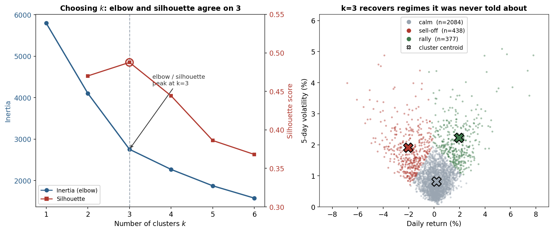
Both diagnostics agree the data wants three clusters: the inertia curve elbows at k=3 (falling 5798 → 4105 → 2756 before flattening) and the silhouette score peaks there (0.49). And the three groups it finds are not arbitrary — they are regimes any trader would recognise. A large calm cluster (2,084 days, average return +0.18%, volatility 0.82%) is the everyday market; a sell-off cluster (438 days, −2.04% return, 1.90% volatility) collects the sharp down days; a rally cluster (377 days, +1.94% return, 2.23% volatility) collects the sharp up days. The classic V-shape in the right panel — big moves of either sign living in high volatility — falls straight out of unlabelled data.
Better still, the clusters persist, which is what makes them regimes rather than labels for yesterday. A day in the calm cluster is followed by an average absolute move of 0.79%; a day in either turbulent cluster is followed by 1.41% — 1.8× larger. This is the same volatility-clustering signal the supervised models found, arrived at from the opposite direction: the random forest was told which days were volatile and learned to predict them; K-means was told nothing and discovered the same structure. What it still can’t do, of course, is tell you which wing tomorrow lands in — the sell-off and rally clusters are symmetric because direction remains unpredictable.
8. What does the Python code look like?
from sklearn.cluster import KMeans
from sklearn.preprocessing import StandardScaler
from sklearn.metrics import silhouette_score

X = StandardScaler().fit_transform(features)      # ALWAYS scale — K-means is distance-based

# choose k: elbow (inertia) + silhouette
for k in range(2, 7):
    km = KMeans(n_clusters=k, n_init=10, random_state=0).fit(X)
    print(k, km.inertia_, silhouette_score(X, km.labels_))

km = KMeans(n_clusters=3, n_init=10, random_state=0).fit(X)   # k-means++ init by default
km.cluster_centers_          # the centroids — each cluster's "average member"
km.labels_                   # cluster assignment per point
n_init runs Lloyd’s several times and keeps the lowest-inertia result (guarding against bad starts); random_state fixes it. The two lines that matter most are the StandardScaler (omit it and the largest-unit feature hijacks the distance) and the loop that justifies your choice of k.
9. How would I explain it to a supervisor?
“K-means is unsupervised — no labels. It partitions the data into k groups by minimising the total squared distance from each point to its cluster centroid, which is the within-cluster variance, using Lloyd’s algorithm: assign points to the nearest centroid, move each centroid to its points’ mean, repeat. You choose k with the elbow and silhouette, scale the features because it’s distance-based, and restart it because it only finds a local optimum. It assumes round, comparable clusters, so it fails on elongated or nested ones. On the Nasdaq I clustered days by return and volatility with no labels, and both diagnostics chose three clusters — a calm core and symmetric sell-off and rally wings — and those regimes persist, a 1.8× difference in next-day volatility. It rediscovered, unlabelled, the volatility-clustering structure the supervised models were trained to find.”
Nasdaq-100 index from the same multi_daily.csv as the Equation Library (yfinance, adjusted closes), ~2,900 daily observations. Days clustered on two standardised features (daily return, 5-day rolling volatility) with scikit-learn KMeans (k-means++, n_init=10). Elbow, silhouette, cluster statistics, and next-day-volatility persistence were computed directly and checked; the six-point Lloyd’s example is worked by hand above.