LightGBM

Gradient boosting, made fast — leaf-wise growth and histogram binning

LightGBM is gradient boosting like XGBoost, but with leaf-wise tree growth and histogram-based splits that make it 25–50× faster at the same accuracy. What’s different, why it’s faster, and when leaf-wise growth overfits.

LightGBM is the same algorithm as XGBoost — gradient-boosted decision trees — with a different engine under the hood. Two engineering choices, leaf-wise tree growth and histogram-based split finding, make it dramatically faster and lighter on large datasets while matching the accuracy. It and XGBoost are the two models that dominate serious tabular machine learning; the choice between them is mostly about data size and how carefully you tune. This entry is short by design: everything about why boosting works is in the XGBoost page — here we cover only what’s different.

1. What problem does it solve?

The same classification and regression on tabular data as XGBoost, aimed at the case where training speed and memory matter: large datasets, wide feature sets, or frequent retraining. When a gradient-boosting model is the right choice and the data is big, LightGBM is usually the faster way to get it.

2. What assumptions does it make?

The same as any gradient-boosted trees — additive weak learners, nonparametric, no scaling — plus one implementation assumption: that binning each continuous feature into a few hundred discrete buckets loses negligible accuracy. In practice it does, and it buys a large speed-up.

3. What data does it need?

Tabular data, and it shines when that data is large — hundreds of thousands to millions of rows. It handles categorical features natively (no one-hot encoding) and copes with missing values. The one caution is the opposite of its strength: on small datasets, its aggressive leaf-wise growth overfits easily, so on little data a more conservative model (or heavy regularisation) is safer.

4. How does it learn?

The boosting core is identical to XGBoost — fit each new tree to the negative gradient of the loss, add it with a learning rate. Two things differ, both about how the trees are built:

• Leaf-wise (best-first) growth. XGBoost grows a tree level by level, splitting every node at each depth (balanced). LightGBM instead splits the single leaf that promises the largest loss reduction, wherever it is — producing deep, lopsided trees that lower the loss faster per split. The figure shows the contrast. The cost is overfitting risk, controlled by capping num_leaves and min_data_in_leaf.
• Histogram-based splits. Rather than sorting every feature value to find a split, LightGBM buckets each feature into ~255 bins once, then searches over bins. That turns split-finding from O(\text{rows}) into O(\text{bins}), which is the bulk of the speed-up and the memory saving.

Two further tricks sharpen it: GOSS (keep the high-gradient examples, subsample the low-gradient ones — focus on the hard cases) and EFB (bundle mutually-exclusive sparse features into one). The output is the same kind of additive tree ensemble; it is just built far more cheaply.

5. What are its strengths?

• Speed and low memory. Often an order of magnitude faster than level-wise boosting — 25–51× in the test below — with the gap widening as data grows.
• Same accuracy. It matches XGBoost’s predictive quality; you pay nothing for the speed.
• Native categoricals. No one-hot blow-up; it splits categorical features directly.
• Scales. Comfortable on datasets far too large for exact, sort-based boosting.
• Fast iteration. When each fit is seconds not minutes, you can tune and cross-validate properly.

6. What are its weaknesses?

• Leaf-wise growth overfits small data. Its greatest strength on big data is a liability on small; cap num_leaves, raise min_data_in_leaf, and regularise.
• More sensitive hyperparameters. The extra knobs (num_leaves, bin count, GOSS settings) need care.
• Binning is approximate. Histogram splits sacrifice a little precision for speed (usually worth it).
• Same black-box and early-stopping caveats as XGBoost. It overfits without a validation stop, and hundreds of trees aren’t interpretable.

7. How could it apply to markets?

Wherever you’d use XGBoost for a tabular quant signal but the data is large — a deep history of high-frequency bars, a broad cross-section of assets crossed with many features, or a pipeline that retrains often — LightGBM gets you the same model faster. The same discipline applies: early stopping, walk-forward validation, and, because leaf-wise growth overfits noise so readily, a firm cap on num_leaves when the signal-to-noise is as low as it is in finance.

Left: level-wise growth (XGBoost) splits every node at each depth for a balanced tree; leaf-wise growth (LightGBM) splits the best leaf first, going deep and asymmetric — faster to lower the loss. Right: training time (log scale) — LightGBM is 25× faster on the Nasdaq volatility task and 51× on a 40k-row synthetic set, at essentially equal AUC.

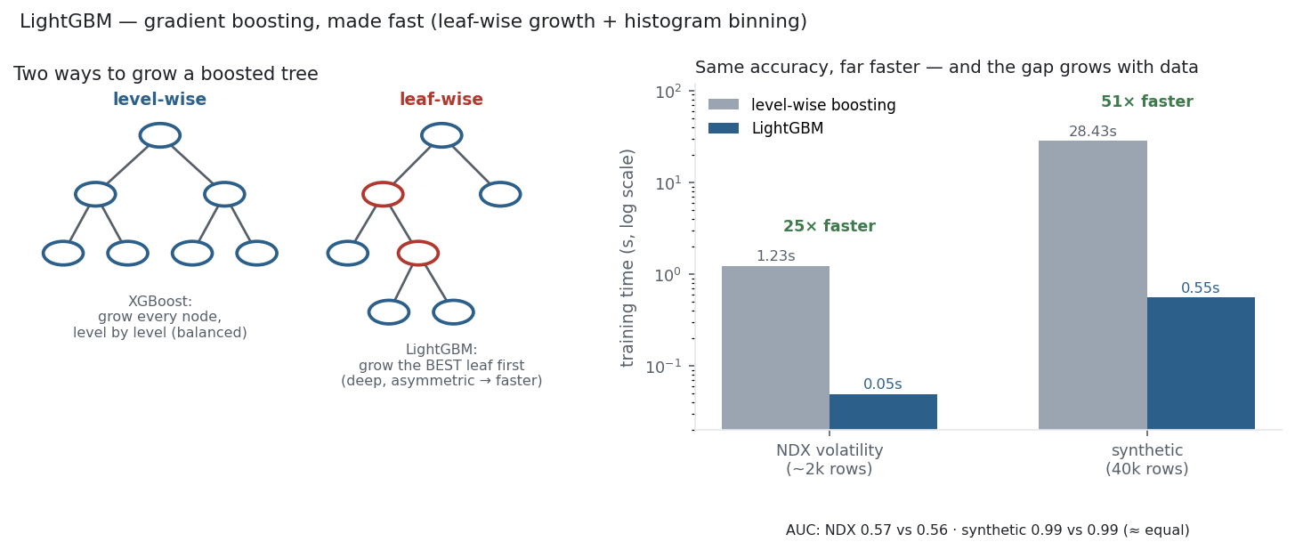
On the same volatility-clustering task as the earlier tree models, LightGBM lands the same test AUC (≈0.57) as level-wise boosting but trains in 49 milliseconds versus 1.2 seconds — 25× faster. Scale the problem up to a 40,000-row synthetic dataset and the gap widens to 51× (0.55s versus 28s), at identical accuracy (0.99 AUC each). That is the whole LightGBM story in one chart: nothing gained or lost in predictive quality, a large and growing saving in time and memory. On a small, near-signal-free task like Nasdaq direction it won’t find what isn’t there any more than XGBoost did — but when there is signal and the data is big, it finds it faster.

8. What does the Python code look like?

import lightgbm as lgb

model = lgb.LGBMClassifier(
    n_estimators=1000, learning_rate=0.05,
    num_leaves=31, min_child_samples=50,          # leaf-wise growth controls (anti-overfit)
    subsample=0.8, colsample_bytree=0.8, reg_lambda=1.0)
model.fit(X_train, y_train, eval_set=[(X_val, y_val)],
          callbacks=[lgb.early_stopping(50)])       # stop when validation stalls
# categorical_feature=[...] to use native categorical splits (skip one-hot)

num_leaves is the knob — it replaces max_depth as the complexity control, and on noisy data you keep it modest. Everything else mirrors XGBoost.

9. How would I explain it to a supervisor?

“LightGBM is gradient boosting, same as XGBoost, but built for speed: it grows trees leaf-wise — splitting the highest-loss leaf first instead of a whole level — and finds splits on histogram bins rather than sorted values. That makes it 25 to 50 times faster and much lighter, with the advantage growing as the data grows, at the same accuracy — I measured both on the Nasdaq volatility task and a larger synthetic one. The trade-off is that leaf-wise growth overfits small or noisy data, so I cap num_leaves and use early stopping. On large tabular problems it’s my default; on small ones I’d reach for XGBoost or regularise hard.”

Nasdaq-100 basket from the same multi_daily.csv as the Equation Library (yfinance, adjusted closes). Timings compare lightgbm against scikit-learn’s level-wise GradientBoostingClassifier on the volatility task and a make_classification synthetic set; AUC and wall-clock times were measured directly and checked.