XGBoost (Gradient Boosting)
Trees built one at a time, each fixing the last one’s errors — the tabular-data champion
The random forest built its trees independently and averaged them, cutting variance. Gradient boosting does the opposite: it builds trees one at a time, each new tree trained to fix the errors the current ensemble still makes. Where bagging is a committee voting in parallel, boosting is a relay — every runner starts where the last left off. Done carefully it produces the most accurate models on tabular data, which is why XGBoost (and its cousin LightGBM) win a huge share of Kaggle competitions and power a great deal of production quant ML. Done carelessly it overfits with a vengeance, and the Nasdaq shows exactly how.
1. What problem does it solve?
The same classification and regression as trees and forests, but pursuing maximum accuracy rather than robustness. It is a boosting ensemble: a sequence of weak learners (shallow trees) combined into one strong predictor. On structured/tabular data it is usually the best-performing model class available — the default first reach for a serious tabular problem.
2. What assumptions does it make?
The same non-assumptions as trees (nonparametric, no scaling, axis-aligned splits), plus the additive premise that a sum of many small trees can approximate the target — which, given enough rounds, can approximate almost anything. That flexibility is also the danger: with no restraint it will approximate the noise too.
3. What data does it need?
Tabular data with mixed types; XGBoost handles missing values natively and needs no scaling. Above all it needs a validation set (or cross-validation): because it keeps improving the training fit indefinitely, you must watch a held-out score to know when to stop.
4. How does it learn?
By gradient boosting — gradient descent, but in function space. Start with a constant prediction, then at each round m fit a shallow tree h_m to the negative gradient of the loss with respect to the current predictions (the “pseudo-residuals” — for squared error, simply the leftover residuals), and add it, shrunk by a learning rate \eta:
F_m(x) = F_{m-1}(x) + \eta\, h_m(x).
Each tree is one step downhill on the loss, exactly as in gradient descent — only the “parameter” being updated is the whole function. XGBoost is the optimised, regularised realisation of this idea: it uses second-order gradient information (the Hessian, not just the slope), adds L1/L2 penalties on the leaf weights, shrinks each tree by \eta, subsamples rows and columns per tree, and prunes — a stack of regularisers precisely because raw boosting overfits so easily. Where a forest reduces variance, boosting reduces bias, building a low-error model out of high-bias stumps.
5. What are its strengths?
- Best-in-class accuracy on tabular data. It routinely beats forests, SVMs, and neural nets on structured problems.
- Captures complex structure. Deep interactions and nonlinearities emerge from stacking many small trees.
- Heavily regularised (XGBoost). Shrinkage, L1/L2, subsampling and pruning give fine control over the bias-variance trade.
- Handles missing values and mixed types. No imputation or scaling needed.
- Efficient and battle-tested. XGBoost/LightGBM are highly optimised and parallelised within each tree.
6. What are its weaknesses?
- Overfits without early stopping. It will drive training loss to zero and generalisation with it — you must stop on a validation score.
- Many hyperparameters. Learning rate, depth, rounds, subsampling, and regularisation all interact and need tuning.
- Sensitive to noisy labels. Because each tree chases the current errors, it happily fits mislabelled or random points.
- Less interpretable. Hundreds of sequential trees are a black box (use SHAP and importances).
- Still can’t invent signal. More rounds fit more noise, not more truth — the bias reduction only helps where structure exists.
7. How could it apply to markets?
XGBoost is the default engine for serious tabular quant work: fusing dozens of price, volume, and alternative-data features into a signal; predicting volatility or regimes; ranking a cross-section of assets — always with early stopping and walk-forward validation, because financial data is exactly the noisy, low-signal regime where boosting overfits.
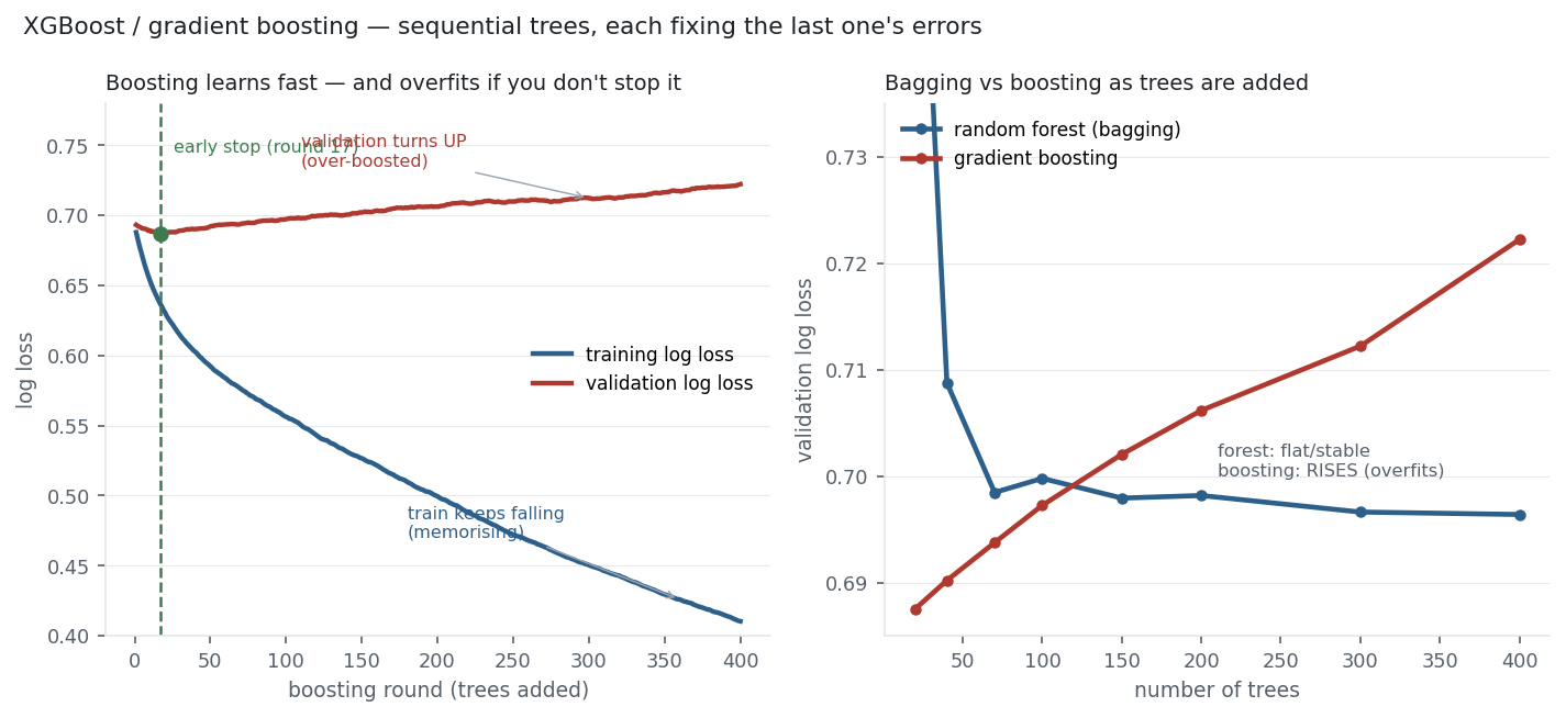
Boosted on the same volatility-clustering task as the forest — predicting a high-volatility day from the last ten absolute returns — gradient boosting reaches a test AUC of about 0.57, matching the random forest and confirming the signal is real. But the left panel is the lesson unique to boosting: the training log loss falls without limit as trees are added (0.69 → 0.41, memorising the training set), while the validation log loss bottoms out at round 17 and then rises. Left to run 400 rounds it overfits badly. The right panel drives the bagging-vs-boosting distinction home: pile more trees on a random forest and it stays flat (safe); pile them on gradient boosting and it gets worse. Boosting is more powerful and more dangerous — which is why early stopping isn’t optional.
8. What does the Python code look like?
import xgboost as xgb

model = xgb.XGBClassifier(
    n_estimators=1000, learning_rate=0.05, max_depth=3,
    subsample=0.8, colsample_bytree=0.8,
    reg_lambda=1.0, reg_alpha=0.0,            # L2 / L1 on leaf weights
    early_stopping_rounds=50, eval_metric="logloss")
model.fit(X_train, y_train, eval_set=[(X_val, y_val)])   # stops when val stops improving
print(model.best_iteration)                               # the early-stop round
learning_rate (shrinkage) and early_stopping_rounds are the two knobs that matter most; smaller \eta with more rounds and early stopping is the standard recipe. sklearn’s HistGradientBoostingClassifier is a fast, dependency-free alternative.
9. How would I explain it to a supervisor?
“Gradient boosting builds shallow trees sequentially, each one fit to the negative gradient of the loss given the current model — it’s gradient descent in function space, with a learning rate. XGBoost is the regularised, second-order version: L1/L2 on the leaves, shrinkage, row and column subsampling. It’s the strongest tabular model and reduces bias, where a forest reduces variance. On the Nasdaq it recovers the same 0.57 volatility AUC as the forest — but its validation loss bottoms at 17 rounds and then climbs, so unlike bagging it overfits with more trees. That’s why I always pair it with a learning rate and early stopping, and validate walk-forward on market data.”
Nasdaq-100 basket from the same multi_daily.csv as the Equation Library (yfinance, adjusted closes). Learning curves from scikit-learn GradientBoostingClassifier (the same algorithm as XGBoost) on the volatility task, 70/30 time split; the random-forest comparison and the early-stop round were computed and checked.