Overfitting in Trading Systems

Try enough strategies and one looks brilliant by luck — backtest overfitting and how to deflate it

Even with clean data, no leakage, and honest validation, searching over many strategies inflates the best in-sample performance. The maximum-of-N mechanism, why in-sample rank says nothing about out-of-sample, the deflated Sharpe ratio, and the probability of backtest overfitting.

The leakage page fixed bugs inside a single backtest. This is a deeper failure that survives all of that. Suppose every individual backtest is methodologically perfect — clean data, no leakage, honest walk-forward. If you nonetheless try enough strategies and keep the best one, that winner is overfit: it looks brilliant in-sample purely because you searched, and it delivers nothing out of sample. This is backtest overfitting through multiple testing, and it is the single most common reason a spectacular backtest becomes a losing live strategy. It is also the most seductive, because the good-looking result is exactly the one you were hoping to find.

1. What problem does it solve?

It names and quantifies selection bias under multiple testing. When you search over many strategies, parameters, features, or models and report the best in-sample performer, that reported performance is inflated — the maximum of many noisy estimates is biased upward even when no strategy has any real edge. The failure is not in any single backtest, each of which may be flawless; it is in the act of selecting the best across many. Recognising it, and adjusting for it, is what separates a real edge from a lucky draw.

2. When does it bite?

Whenever you search: tuning parameters, trying many signals or feature sets, comparing models, or — worst — mining combinations at scale. The more configurations you try, the more inflated the winner. It is amplified by the short samples typical of finance (a few years of daily data make every Sharpe estimate noisy) and it hides in plain sight precisely because each individual backtest can be perfect. The insidious part is that your true trial count includes every tweak and every abandoned idea across the whole research history — the “garden of forking paths”.

3. What is the mechanism?

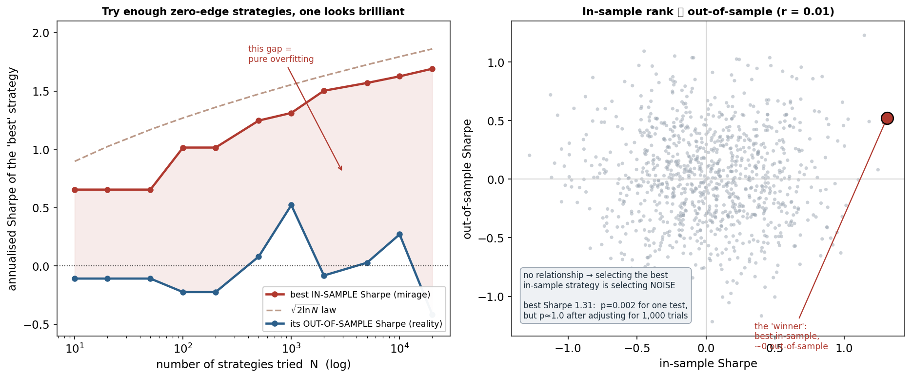
The maximum of N noisy estimates. A zero-edge strategy’s in-sample Sharpe is a noisy estimate whose standard error is roughly \sqrt{\text{periods per year}/T} — here about 0.42 annualised over half the Nasdaq sample. The expected maximum of N such estimates grows like \sqrt{2\ln N} times that standard error, so it climbs steadily with every strategy you try. The left panel shows it directly: taking N random, edgeless long/short strategies on real Nasdaq returns, the best in-sample Sharpe rises from 0.65 at N=10 to 1.02, 1.31, and 1.63 at N=100, 1{,}000, and 10{,}000 — a “hireable” number conjured from pure luck — while the very same strategy’s out-of-sample Sharpe hovers around zero. The right panel is the killer: across a thousand strategies the in-sample and out-of-sample Sharpe are uncorrelated (r = 0.01). In-sample rank tells you nothing about out-of-sample performance, so picking the in-sample best is picking noise.

Left: the best in-sample Sharpe of N random zero-edge strategies climbs with N, tracking the \sqrt{2\ln N} law, while the same strategy’s out-of-sample Sharpe stays near zero — the shaded gap is pure overfitting. Right: in-sample versus out-of-sample Sharpe for 1,000 strategies shows no relationship (r=0.01); the in-sample “winner” (red) has essentially no out-of-sample edge, and its Sharpe of 1.31 — significant at p = 0.002 for a single test — is worthless (p ≈ 1) after adjusting for 1,000 trials.

4. How do you detect and defend against it?

The defences all come down to accounting for how hard you looked:

• Count your trials and adjust. The winning Sharpe of 1.31 has a single-test p-value of 0.002 — apparently significant — but after adjusting for 1,000 trials it is p ≈ 1, entirely insignificant. Even crude Bonferroni is better than ignoring the search.
• Deflated Sharpe ratio (Bailey & López de Prado). It corrects the observed Sharpe for the number of trials, the sample length, and the returns’ skew and kurtosis, answering: is this Sharpe significant given how many I tried?
• Probability of backtest overfitting (PBO) via combinatorially symmetric cross-validation — the probability that the in-sample-best configuration underperforms the median out of sample. It is the natural companion to the time-series CV distribution: a high PBO means your selection is capturing noise.
• Search less, and lock a test set. Prefer few, theory-driven hypotheses over mass mining; hold out a truly untouched period, use it once, and report the trial count honestly.

5. What are its strengths (as a discipline)?

• Turns “great backtest” into “great backtest given N trials” — the only honest way to read a search result.
• Quantifiable. The deflated Sharpe and PBO put a number on the overfitting risk rather than leaving it to intuition.
• Prevents the most expensive mistake in quant — deploying a strategy whose entire edge was selection luck.
• Cheap awareness. Simply tracking and reporting the number of configurations tried changes how a result is judged.

6. What are its weaknesses (and difficulties)?

• The true trial count is usually unknown. Every tweak, discarded idea, and intuition-guided choice counts, and no one records them all.
• Short samples make it worse. Financial history is limited, so estimates are noisy and the maximum-of-N inflation is large.
• Defences reduce, not eliminate. Deflated Sharpe and PBO are estimates with their own assumptions.
• Explore-versus-honesty tension. Good research requires trying things; honesty requires paying for each trial — the two pull against each other.
• It is psychologically hard. The overfit backtest is the one you want to be real, which is exactly why it fools people.

7. How could it apply to markets?

This is arguably the central pitfall of quantitative strategy research, and the demonstration is the whole warning: random, edgeless strategies produce Sharpe-1.6 backtests if you try ten thousand of them, and the in-sample champion has zero out-of-sample edge. Because genuine edges are small and rare — the efficient-market thread running through this entire site — the base rate is that a great-looking backtest is overfit, so the correct prior is skepticism and the correct action is to deflate hard. For a MarketLens signal: track how many configurations you tried, deflate the Sharpe for that count, compute PBO with combinatorial purged CV, keep a locked-away test period you touch once, and treat any strategy discovered by search as guilty until it survives that scrutiny. The models earlier in this library found volatility structure and no direction edge; the discipline here is what stops you from believing a direction edge that a thousand trials manufactured from noise.

8. What does the Python code look like?

import numpy as np
# The maximum-of-N mirage: N random zero-edge strategies on real returns
def best_of_n(returns, N, T_is, ann=np.sqrt(252)):
    pos = np.random.choice([-1, 1], size=(N, len(returns)))    # random long/short, NO edge
    sret = pos * returns
    sharpe = lambda x: x.mean() / x.std() * ann
    is_sh  = np.array([sharpe(sret[i, :T_is]) for i in range(N)])
    best   = is_sh.argmax()
    oos_sh = sharpe(sret[best, T_is:])
    return is_sh[best], oos_sh          # best in-sample looks great; out-of-sample ~ 0

# deflate for trials: a single-test p-value must be adjusted for how many you ran
from scipy.stats import norm
def is_it_real(observed_sharpe, T, n_trials, ann=np.sqrt(252)):
    t = observed_sharpe / (ann * np.sqrt(1 / T))               # standardise vs the null
    p_single = 2 * (1 - norm.cdf(abs(t)))
    return min(1.0, p_single * n_trials)                       # ~Bonferroni; use DSR for rigour

The honest workflow is to record n_trials, deflate accordingly, and never trust a searched-for Sharpe at face value. Libraries like mlfinlab implement the deflated Sharpe ratio and PBO directly.

9. How would I explain it to a supervisor?

“Backtest overfitting is selection bias: if you try enough strategies and keep the best, its in-sample performance is inflated even when nothing has a real edge, because the maximum of many noisy Sharpe estimates grows like the square root of two-log-N. I showed it — random, edgeless strategies on Nasdaq returns give a best in-sample Sharpe rising from 0.65 to 1.63 as you go from 10 to 10,000 trials, while their out-of-sample Sharpe stays at zero and in-sample rank is uncorrelated with out-of-sample, r of 0.01. A Sharpe of 1.31 looks significant at p = 0.002 for one test but is p ≈ 1 after adjusting for a thousand trials. The defences are to count trials and deflate — the deflated Sharpe ratio — and to compute the probability of backtest overfitting with combinatorial cross-validation. It’s distinct from leakage: every individual backtest can be clean and you still overfit by cherry-picking, so I track the trial count, keep a test set I touch once, and stay skeptical of anything found by search.”

N random long/short daily strategies (independent \pm 1 positions, no edge) on Nasdaq-100 returns from the same multi_daily.csv as the earlier entries; 50/50 in-sample/out-of-sample split; annualised Sharpe. Per-strategy in-sample Sharpe standard deviation 0.418 (theory \sqrt{252/T}=0.417); best-of-N Sharpe, in-sample/out-of-sample correlation, and the multiple-testing p-value adjustment were computed and checked. Every number was verified.