Q-Learning & Deep Q-Networks
Learning optimal decisions from experience alone — checked against the exact answer
The MDP entry solved the regime position-sizing problem exactly — but only because we handed the solver the model: the HMM’s transition matrix and the reward function. A real trading agent has neither. Q-learning is the classic answer to that harder problem: learn the optimal action-values purely from sampled experience — tuples of (state, action, reward, next state) — with no knowledge of P or R at all. And because this library has the exact Q^* from value iteration, this entry can do something textbook demonstrations rarely can: run model-free learning and check it against the known ground truth. Three learners — tabular, tabular-behaving-randomly, and a DQN-style neural network — all recover the exactly optimal policy.
1. What problem does it solve?
Model-free control: finding the optimal policy of an MDP whose transition dynamics and rewards are unknown, from interaction alone. This is the realistic setting — markets do not publish their transition matrix — and it is the gap between the MDP formalism and a deployable agent. Q-learning learns Q^*(s,a), the value of taking action a in state s and acting optimally afterwards; once Q^* is known, the optimal policy is just \arg\max_a Q^*(s,a) — no model ever required.
2. What is the update rule?
One line, run on every experienced transition (s, a, r, s'):
Q(s,a) \;\leftarrow\; Q(s,a) \;+\; \alpha\Big[\, r + \gamma \max_{a'} Q(s',a') \;-\; Q(s,a) \,\Big].
The bracket is the temporal-difference (TD) error: the gap between the current estimate and a one-step bootstrapped target — observed reward plus the discounted value of the best next action. Each update nudges Q toward a sampled version of the Bellman optimality equation; the expectation over s' that value iteration computed from P is here replaced by the environment’s own samples. Under standard conditions (every pair visited infinitely often, step sizes decaying appropriately), tabular Q-learning converges to Q^* — the stochastic-approximation cousin of the Bellman contraction.
3. Why is “off-policy” the superpower?
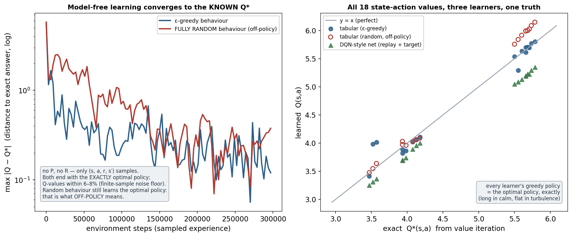
The \max_{a'} in the target means Q-learning always evaluates the greedy policy — regardless of how the data was generated. The behaviour policy (what the agent does, e.g. ε-greedy exploration) and the target policy (what it learns about, the optimal one) are decoupled. The demonstration makes this vivid: a learner that behaves completely at random — never once exploiting what it knows — still converges to the same Q^* and the same optimal policy as the ε-greedy learner (left panel, red). For finance this property is not a curiosity but the whole game: you cannot explore markets by trading randomly with real money, so learning from data generated by some other process — history, a different strategy, a simulator — is the only viable mode. Off-policy learning, taken to its limit, is offline RL: learning from a fixed historical dataset, the setting my PhD proposal targets.
4. What did the demonstration show?
The environment is the regime MDP from the previous entry — HMM regime dynamics, exposure actions, risk-adjusted reward with switching costs — but the learners see only samples. Results, all checked against the exact Q^*:
- Tabular, ε-greedy: after 300k sampled steps, the greedy policy exactly matches the optimal policy (fully long in calm, flat in turbulence), with Q-values within 8.0% of Q^* — a finite-sample noise floor, not bias.
- Tabular, fully random behaviour: same result — policy exactly optimal, values within 6.3% — despite never acting greedily. Off-policy, demonstrated.
- DQN-style network (a small neural Q-network trained with the two tricks that made deep Q-learning work — an experience replay buffer that decorrelates samples, and a periodically-frozen target network that stabilises the bootstrapped target): policy exactly optimal, values within 8.3%.
The DQN run also surfaced a lesson worth recording. With the target network refreshed too rarely, learning stalled at a large error — because each refresh propagates roughly one Bellman sweep, so 112 refreshes cannot do the work of value iteration’s thousands. Refreshing more frequently fixed it. The target network is a dial between stability (stale targets don’t chase themselves) and speed (stale targets slow value propagation) — a trade-off you can see, not just recite.
5. What are its strengths?
- No model needed. It learns optimal behaviour from raw interaction — the setting real decision problems actually present.
- Off-policy. It learns the optimal policy from data generated any other way — exploration, history, another strategy — the property finance cannot do without.
- Provably convergent (tabular). With sufficient visitation and decaying steps, convergence to Q^* is a theorem, and the demonstration hits it.
- Scales via function approximation. DQN replaces the table with a network, extending the idea to state spaces where tables are impossible — Atari from pixels was this exact algorithm.
- Simple and auditable. One update rule; the learned Q is inspectable state by state, as the scatter shows.
6. What are its weaknesses?
- The deadly triad. Function approximation + bootstrapping + off-policy learning can diverge; DQN’s replay buffer and target network are engineering patches, not guarantees.
- Sample-hungry. Even this 6-state problem took hundreds of thousands of samples for tight values — real state spaces need vastly more, a serious constraint when data is finite market history.
- Maximisation bias. The \max over noisy estimates is biased upward (double Q-learning is the fix).
- Discrete actions. Vanilla Q-learning needs \arg\max_a over a finite set; continuous exposure requires the policy-gradient family — the next entry.
- Values ≠ certainty. The 6–8% value error is harmless here because the policy is preserved; with closer-valued actions, that noise flips decisions.
7. How could it apply to markets?
This entry is the first learning component of the PhD proposal’s RL Trading Agent, and its lessons transfer directly. The off-policy property is the licence to learn from history rather than live experimentation — but its honest limit must be stated equally clearly: learning from a fixed dataset (offline RL) cannot try actions the data never took, so counterfactuals are extrapolated, not observed, and modern offline-RL methods exist precisely to restrain that extrapolation. The sample-hunger finding is a market-sized warning: a toy problem needed 300k transitions while a decade of daily data offers ~2,500 — which is why the proposal’s agent operates on regime beliefs and engineered features (a small, structured state) rather than raw market history, and why its rewards are risk-sensitive rather than raw P&L. And the ground-truth check performed here is a discipline worth keeping: before trusting any RL agent on markets, verify the machinery recovers a known optimum on a solvable problem — the RL equivalent of this site’s gradient checks.
8. What does the Python code look like?
import numpy as np

Q = np.zeros((n_states, n_actions))
alpha, gamma, eps = 0.5, 0.99, 0.2

s = env.reset()
for t in range(300_000):
    a = env.random_action() if np.random.rand() < eps else Q[s].argmax()   # behaviour policy
    r, s2 = env.step(s, a)                       # sampled experience — no P, no R known
    td_target = r + gamma * Q[s2].max()          # bootstrapped Bellman target (off-policy max)
    Q[s, a] += alpha * (td_target - Q[s, a])     # the one-line update
    s = s2
policy = Q.argmax(axis=1)                        # greedy in learned Q  ->  optimal policy

# DQN = same update with a network Q(s,a; θ), plus:
#   replay buffer  — sample past transitions i.i.d. (decorrelates the data)
#   target network — freeze θ⁻ for the bootstrap target (stabilises what you chase)
The tabular loop is genuinely this short. The DQN additions exist because a network chasing its own moving predictions is unstable — replay and target networks are what made the idea work at scale.
9. How would I explain it to a supervisor?
“Q-learning learns the optimal action-value function of an MDP without knowing its dynamics: on every sampled transition it nudges Q(s,a) toward the reward plus the discounted max over next actions — a stochastic version of the Bellman optimality update. The max makes it off-policy: it learns the optimal policy regardless of how the data was generated, which I demonstrated by having an agent behave completely at random and still recover the exact optimal policy. Because I’d solved the same regime MDP exactly, I could verify convergence against ground truth — tabular and a small DQN with replay and a target network all matched the optimal policy exactly, values within eight percent. The DQN run also showed the target-network trade-off directly: refresh too rarely and each refresh only propagates one Bellman sweep, so learning stalls. For markets, off-policy is the licence to learn from historical data — offline RL — but the sample-hunger is the binding constraint, which is why my proposal keeps the state small and structured. Continuous actions need policy gradients, which is the next entry.”
Environment: the regime MDP (fitted HMM dynamics, exposure actions, risk-adjusted reward, \gamma=0.99, c=10bp), simulated; exact Q^* from value iteration to 10^{-12}. Tabular Q-learning: 300k steps, decaying step size, ε=0.2 and fully-random behaviour. DQN-style learner: one-hot inputs, 24-unit hidden layer, replay buffer (30k), target network (150-step refresh), trained by SGD. All final policies match the optimal policy exactly; value errors 6.3–8.3% of \max|Q^*|. Every number was checked.