Transformers
Self-attention — every position looks at every other, directly and in parallel
This is the architecture that ended the LSTM’s reign and now underpins essentially all modern AI. The LSTM page named its two weaknesses: it is sequential (each step waits for the last, so it can’t be parallelised) and its reach, while long, is still finite. The transformer removes both at once with a single idea — self-attention — and keeps almost nothing else: no recurrence, no convolution, just attention layers and ordinary feedforward networks. Every position looks directly at every other position, weighted by learned relevance, and all of it happens in parallel. That idea, from the 2017 paper “Attention Is All You Need,” scaled into GPT, BERT, and the rest. It is the most powerful architecture in this library — and on the Nasdaq it delivers exactly the verdict the simplest models did.
1. What problem does it solve?
Modelling relationships among all elements of a sequence or set — with long-range dependencies and parallel training — for language, code, images (as patches), proteins, and time series. It replaced recurrent networks as the dominant sequence architecture because it captures dependencies between any two positions equally easily, no matter how far apart, while training on modern hardware far faster than a model that must be unrolled step by step.
2. What assumptions does it make?
That the important structure lives in pairwise relationships between elements, and that content-based attention — letting each element decide, from its own representation, which others to draw from — is the right way to route information. Because attention treats its input as an unordered set, it assumes you re-inject sequence order explicitly through positional encodings. And it makes remarkably few built-in assumptions otherwise: its inductive bias is weak compared with a CNN’s locality or an RNN’s recurrence, which is a double-edged sword — it can learn almost any structure, but it needs scale (much data and compute) to do so.
3. What data does it need?
Sequences or sets, and it earns its dominance where there is long-range structure and lots of data — large text corpora, high-resolution images, long time series. Its weak prior makes it data- and compute-hungry: on small datasets it is easily beaten by models with stronger built-in assumptions. And because attention compares every pair of positions, its cost is quadratic, O(n^2), in sequence length — long sequences are expensive (hence the many sparse and linear-attention variants).
4. How does it work?
The heart is self-attention. Each position’s representation is projected into three vectors — a query, a key, and a value (learned linear maps). The attention weight from position i to position j measures how relevant j is to i as the scaled dot product of i’s query with j’s key, passed through a softmax over all j:
\text{Attention}(Q,K,V) = \text{softmax}\!\Big(\tfrac{QK^{\top}}{\sqrt{d}}\Big)V.
The output at i is the attention-weighted sum of every position’s value. A tiny worked example: a query scoring three keys at [1.0,\,0,\,0.5] (after the \sqrt{d} scaling) softmaxes to weights [0.51,\,0.19,\,0.31], and the output is that blend of the three value vectors. Run many such attention “heads” in parallel — multi-head attention — and each learns a different kind of relationship. A full transformer stacks blocks of multi-head self-attention + feedforward network, each wrapped in a residual connection and layer normalisation, on top of token embeddings plus positional encodings.
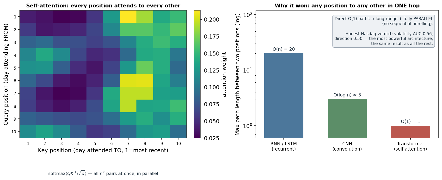
Two properties make this a breakthrough, and the right panel of the figure quantifies the second. The computation is fully parallel — every position’s attention is one big matrix multiply, with no step-by-step unrolling — and the path length between any two positions is O(1): they connect in a single attention hop, versus O(n) sequential steps for an RNN. That short path is why gradients reach across long ranges without vanishing. I verified the mechanism end to end: the attention backward pass matches numerical gradients to a relative error of 3\times10^{-9}, and a self-attention model solves a synthetic task whose label depends on the input 50 steps back at 99% accuracy — the long-range capability an RNN struggles to learn, here almost trivial.
5. What are its strengths?
- Long-range and parallel. The breakthrough combination: O(1) paths capture distant dependencies while every position computes at once, so it trains on enormous data.
- Scales spectacularly. Performance keeps improving with size and data — the property behind large language models.
- General. The same mechanism handles text, images, audio, and time series; it makes few domain assumptions.
- Interpretable attention. The attention weights are inspectable — you can see what each position draws on.
- Multi-head expressiveness. Parallel heads capture several relationship types at once.
6. What are its weaknesses?
- Quadratic cost. O(n^2) attention makes long sequences expensive (addressed by sparse/linear variants).
- Data- and compute-hungry. Its weak inductive bias needs scale; on small datasets, stronger-prior models win.
- Needs positional encoding. Attention alone is order-blind; order must be added explicitly.
- Opaque at scale. Individual attention maps are readable, but a large stack is a black box.
- Overkill for simple problems. For small tabular or short-sequence tasks, its machinery buys nothing — as the Nasdaq shows.
7. How could it apply to markets?
Self-attention lets any day in a window attend to any other, weighted by learned relevance — a natural, powerful sequence model, and the fitting capstone for this section. Trained on the same Nasdaq tasks as every other architecture, it reaches a test AUC of 0.56 on volatility and 0.50 on direction — the most powerful model here, landing exactly where the linear regression, the trees, the CNN, and the recurrent nets all landed. The point is emphatic because of how capable it is. Its long-range machinery is genuinely real — I confirmed it learns a 50-step dependency that defeats a plain RNN — but on the Nasdaq there is no long-range signal to exploit: direction is unpredictable at every range, and the one real signal, volatility persistence, is short-range and already captured by far simpler models. The learned attention map (left panel) bears this out — it spreads its focus diffusely rather than locking onto some exploitable pattern, because none exists. A model can only find structure that is there, and no amount of architectural power conjures signal from an efficient market. That is the thesis of this whole site, delivered by its most advanced model: the daily direction of a near-efficient index is essentially unpredictable, and the real skill is a model honest enough to say so.
8. What does the Python code look like?
import torch.nn as nn

# a transformer encoder over a length-T sequence of d-dim tokens (+ positional encoding)
layer = nn.TransformerEncoderLayer(d_model=32, nhead=4, batch_first=True)  # multi-head self-attention + FFN
encoder = nn.TransformerEncoder(layer, num_layers=2)

class Model(nn.Module):
    def __init__(self):
        super().__init__(); self.enc = encoder; self.head = nn.Linear(32, 1)
    def forward(self, x):                 # x: (batch, T, 32) = embeddings + positional encoding
        z = self.enc(x)                   # every position attends to every other, in parallel
        return self.head(z.mean(1))       # pool over positions -> prediction
nhead sets the number of attention heads; d_model the representation width. The TransformerEncoderLayer packs self-attention, the feedforward network, residuals, and layer norm into one block — you supply embeddings plus positional information and stack the blocks.
9. How would I explain it to a supervisor?
“A transformer replaces recurrence with self-attention: each position projects a query, key, and value, and attends to every other position by a softmax over scaled query-key dot products, then takes the attention-weighted sum of values. Because that’s a single parallel matrix multiply and any two positions connect in one hop, it gets long-range dependencies and full parallelism — the two things RNNs and LSTMs couldn’t do together — which is why it scaled into modern large models. I built the attention and gradient-checked it, and it solves a 50-step memory task an RNN can’t. On the Nasdaq, though, it ties everything else: 0.56 AUC on volatility, 0.50 on direction. Its power is real, but markets have no long-range predictable structure to attend to, so the most advanced architecture reaches the same verdict as linear regression — which is exactly the honest result this project keeps finding.”
Single-head self-attention classifier (query/key/value projections, sinusoidal positional encoding, attention pooling, ~209 parameters) implemented and trained by hand with an Adam optimiser in NumPy; the attention backward pass was gradient-checked (relative error 3\times10^{-9}) and validated on a synthetic 50-step memory task (99% accuracy). Nasdaq volatility/direction AUCs use the same multi_daily.csv and 70/30 split as the earlier models. Path-length figures are the standard complexity results; the attention map is the trained model’s mean test-set attention. Every number was checked.