Recurrent Neural Networks

Processing sequences step by step with a hidden state — memory, and the gradient that won’t reach back

An RNN reads a sequence one step at a time, carrying a hidden state as memory, with the same weights shared across time. Backpropagation through time, the vanishing/exploding gradient that caps its memory, and an honest Nasdaq sequence test.

The convolutional network handles a sequence by sliding a fixed window across it. A recurrent network takes the other, more natural route: it reads the sequence one step at a time, maintaining a hidden state that summarises everything seen so far and updating it at each step. That state is a memory, and the same small “cell” — the same shared weights — is applied at every timestep, so an RNN handles sequences of any length and, in principle, carries information across the whole of it. It is the classic architecture for time series, and a nonlinear generalisation of the autoregressive model you already know. It also has a specific, famous weakness that defines the model after it: the gradient that trains it cannot reach far back in time.

1. What problem does it solve?

Supervised learning on sequences, where order and history carry the signal — time series, language, audio. An RNN maps a variable-length input sequence to an output: to a single label (many-to-one, e.g. classify a return window), to another sequence (many-to-many, e.g. translation), or step-by-step predictions. Conceptually it is a stateful, nonlinear autoregression: where the linear AR model predicts from a fixed weighted sum of past values, an RNN keeps a learned nonlinear summary of the entire past in its hidden state and predicts from that.

2. What assumptions does it make?

That the data is sequential with temporal dependencies worth modelling; that a fixed-size hidden state can adequately summarise the relevant past (the state is assumed sufficient — everything the future needs about the past is compressed into it); and that the same transition governs every timestep — the update from h_{t-1} to h_t uses one shared set of weights, a time-invariance assumption exactly analogous to a CNN’s translation invariance, but along the time axis.

3. What data does it need?

Sequences, and — a real advantage — they can be of variable length, because the same cell is applied however many steps there are. The order must be meaningful (shuffle the timesteps and you destroy the signal). Because the weights are shared across time, the parameter count is independent of sequence length, which is efficient; the difficulty is not parameters but gradients on long sequences, as below.

4. How does it learn?

The recurrence is one equation applied repeatedly:

h_t = \tanh\!\big(W_x\,x_t + W_h\,h_{t-1} + b\big),

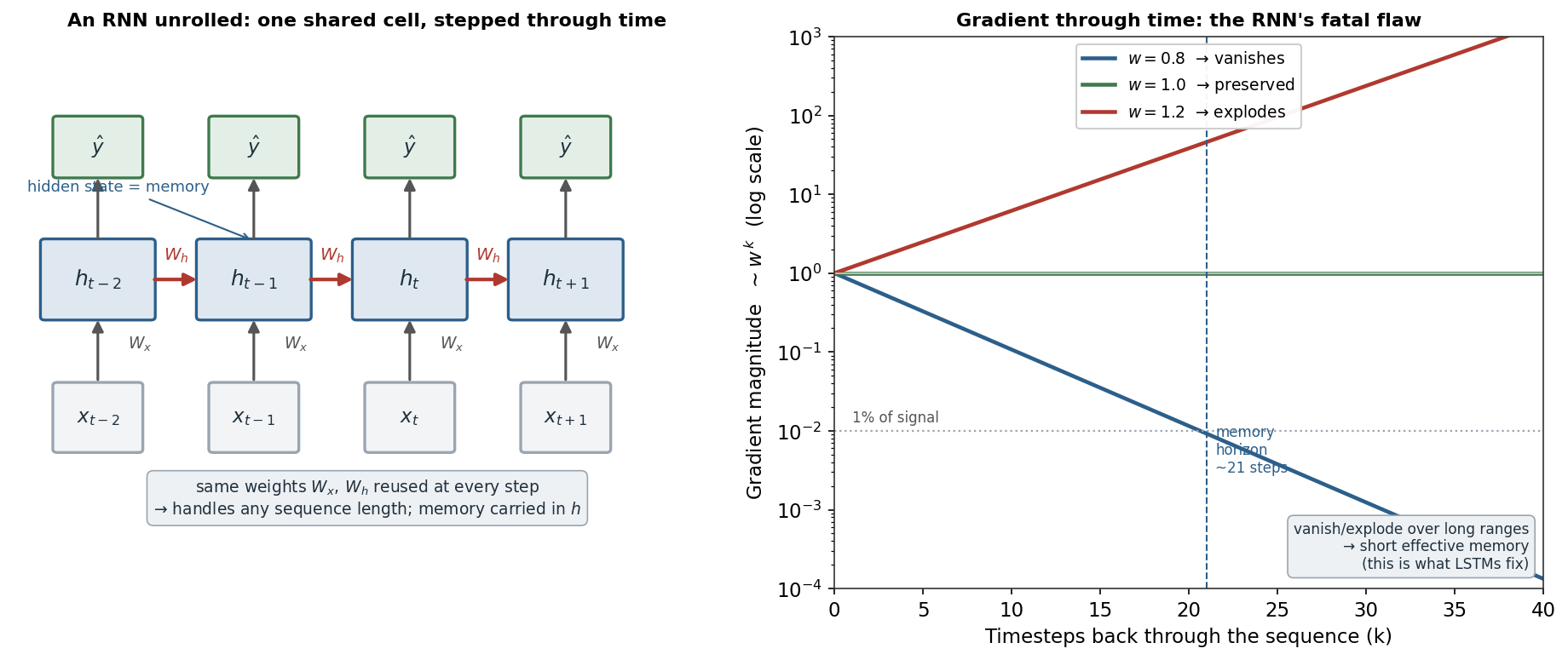
with a prediction read off the final state, \hat y = W_o h_T. The same W_x and W_h are used at every step — weight sharing across time, the left panel of the figure. Training unrolls this into a deep feedforward network — one layer per timestep, with tied weights — and applies ordinary backpropagation; the result is backpropagation through time (BPTT).

Here is the catch, and it is the whole reason the next model exists. The gradient that flows from the loss back to an early step passes through the chain \partial h_T/\partial h_t, which is a product of the per-step Jacobians W_h \odot \tanh' — the same recurrent weight multiplied by itself once per step between. Repeatedly multiplying by one matrix makes the gradient scale like a power, roughly w^{\,k} for k steps back: if the effective recurrent gain is below 1 the gradient vanishes, above 1 it explodes, and only right at 1 is it preserved. The right panel shows all three. With w=0.8 the gradient falls to 1% of its value after ~21 steps — the network’s effective memory horizon — and to 10^{-4} by 40 steps; with w=1.2 it blows up to 10^3. And because \tanh’s derivative never exceeds 1, the multiplier is usually below 1, so vanishing is the common case: a plain RNN simply forgets the distant past. This is the vanishing-gradient problem you met with saturating activations, now unrolled along the time axis — and it is precisely what LSTMs were invented to fix.

Left: an RNN unrolled through time — one shared cell applies the same weights W_x (input) and W_h (recurrent) at every step, passing a hidden state h (the memory) forward. Right: the gradient through time scales like the recurrent weight to the power of the number of steps back. Below 1 it vanishes (a ~21-step memory horizon), at 1 it is preserved, above 1 it explodes — the reason a plain RNN can’t learn long-range dependencies.

5. What are its strengths?

• Built for sequences. Order and history are modelled directly, through a state that evolves step by step — the natural structure for temporal data.
• Variable-length inputs. The same cell processes a sequence of any length, unlike a fixed-input dense net.
• Weight sharing across time. One shared transition means the parameter count doesn’t grow with sequence length — parameter-efficient.
• A genuine memory. The hidden state can, in principle, carry information across arbitrarily many steps.
• The foundation of sequence modelling. RNNs (and their gated successors) drove sequence learning for years before transformers.

6. What are its weaknesses?

• Vanishing/exploding gradients through time. The defining flaw: repeated multiplication by the recurrent weight kills or blows up the gradient, so effective memory is short (~tens of steps).
• Can’t learn long-range dependencies. A direct consequence — distant context is lost before its gradient arrives.
• Sequential and slow. Each step depends on the previous one, so training can’t be parallelised across time the way CNNs and transformers can.
• Sensitive to the recurrent scale. Stability rides on the recurrent weight’s magnitude; gradient clipping and careful initialisation are needed.
• Largely superseded. LSTMs and GRUs fix the memory; transformers fix both memory and parallelism, and now dominate.

7. How could it apply to markets?

An RNN is the natural sequence model for a price series — a nonlinear, stateful autoregression that reads returns in order and keeps a memory. Tested on the same Nasdaq tasks as every other model (a small RNN, 8 hidden units, ~89 parameters, trained by BPTT), it gives the by-now-familiar verdict. On predicting a high-volatility day it scores a test AUC of 0.57 — its running memory of recent absolute returns naturally tracks volatility persistence, matching the forest, boosting, the SVM, and the CNN. On predicting direction it manages AUC 0.52, a hair above a coin flip and well within noise of chance. The stateful memory buys nothing on direction, because signed returns carry no exploitable temporal dependence — and even if some faint long-range structure existed, the ~20-step gradient horizon would keep the RNN from using it. A sequence model, with genuine memory, reaches exactly the conclusion the AR model reached with a handful of linear coefficients: volatility persists and is forecastable; direction is not.

8. What does the Python code look like?

import torch.nn as nn

# a many-to-one RNN over a length-T window of returns (1 feature per step)
rnn = nn.RNN(input_size=1, hidden_size=8, batch_first=True)   # Wx, Wh, b — shared across time
class Model(nn.Module):
    def __init__(self):
        super().__init__(); self.rnn = rnn; self.head = nn.Linear(8, 1)
    def forward(self, x):                 # x: (batch, T, 1)
        _, h = self.rnn(x)                # h: final hidden state (the memory summary)
        return self.head(h.squeeze(0))    # predict from h_T
# loss.backward() runs BPTT; clip gradients (nn.utils.clip_grad_norm_) to tame explosions

hidden_size sets the memory capacity; the parameters (Wx, Wh, b) are shared across all timesteps, so the count is independent of T. Gradient clipping is standard to control the exploding case; the vanishing case is what LSTMs address structurally.

9. How would I explain it to a supervisor?

“An RNN processes a sequence one step at a time, updating a hidden state that acts as memory, using the same weights at every step — weight sharing across time, the temporal analogue of a CNN. You train it by unrolling through the sequence and backpropagating, which is backprop through time. Its defining problem is that the gradient back to early steps is the recurrent weight multiplied by itself once per step, so it scales like that weight to the power of the distance — it vanishes below 1 and explodes above 1, and with tanh it usually vanishes, giving an effective memory of only tens of steps. On the Nasdaq it’s a nonlinear autoregression: 0.57 AUC on volatility, tracking persistence like everything else, and 0.52 on direction, a coin flip. It reaches the same verdict as the linear AR model, and its short-memory flaw is exactly what LSTMs were built to fix.”

RNN (tanh, 8 hidden units, ~89 parameters) implemented and trained by hand with backpropagation through time in NumPy, on the same Nasdaq multi_daily.csv tasks and 70/30 time split as the earlier models; standardised inputs. The gradient-through-time curves are the exact w^{\,k} scaling of the linearised recurrence (tanh bounds the state but the recurrent weight governs the gradient); volatility/direction AUCs were computed and checked.