Does Regime-Conditioning Really Sharpen Tail Probabilities?
Re-testing H2 — this lab’s own surviving positive result — under the protocol that killed the others
H2 was the last standing positive claim in the proposal: that conditioning a tail-probability forecast on the estimated regime beats a volatility benchmark. It was established on one asset, as a 0.002 Brier difference, with no significance test, against a benchmark cruder than the treatment. Re-tested across three indices with a same-information benchmark and Diebold-Mariano tests, not one of six comparisons is significant — and against its own original benchmark the sign reverses on the asset the claim was made on.
Why re-test my own result
By the end of the RQ1 and RQ2 work, a pattern had become impossible to ignore. Every claim that had been put through the full protocol — Diebold-Mariano tests with HAC errors, a deflated significance bar, cross-asset replication, a common scoring window — had weakened or died. And every claim still standing had never been through it.
That is not evidence the survivors are wrong. But it means the proposal’s remaining positive case rested precisely on the results that had not faced the process that killed everything else. So the honest move was to point the process at my own best result first.
H2 is that result: the regime-conditional calibration experiment, which found that conditioning a tail-probability forecast on the estimated regime improves it — and, unlike sizing, beats a volatility benchmark. It is the entire basis for the proposal’s position that the Regime Agent is for calibration, not for sizing.
What was actually claimed
The original reported, on Nasdaq-100 alone, that the Brier score for P(big adverse day) fell from 0.155 (volatility-conditional) to 0.153 (regime-conditional), plus a large improvement in within-regime calibration error.
Two problems with that as evidence, both visible without running anything:
The difference is 0.002, and no significance test was applied. For scale, the largest calibration gain anywhere in the RQ1 panel was −0.0213 at t = −3.93 — ten times bigger — and it still failed to replicate across seven assets.
The benchmark is cruder than the treatment. “Volatility-conditional” meant the expanding event rate inside today’s trailing-volatility tercile — a three-bucket lookup. The regime forecast came from a filtered hidden Markov model. Beating a tercile rule shows that an HMM beats terciles; it does not show that state beats volatility. Avoiding exactly this is what the same-information benchmark in RQ1 exists for.
Data & method
Three indices — NAS100, US500, US30 — daily from 2015, ~1,800 scored days each. Target: the original’s primary one, next day’s return below −1% (base rates 0.114 to 0.185).
Three forecasts, all causal and purged:
- Volatility terciles — the original benchmark, reimplemented: expanding event rate inside today’s trailing-volatility tercile.
- Volatility logistic — the fair benchmark: walk-forward logistic regression on
[rv20, rv60], the same volatility information the regime model sees, used at the same fidelity. - Regime-conditional — the same logistic, plus the filtered HMM state posteriors.
Scored by Brier and compared with Diebold-Mariano using Newey-West errors. Six comparisons, so the deflated bar is \sqrt{2\ln 6} = 1.89.
Results
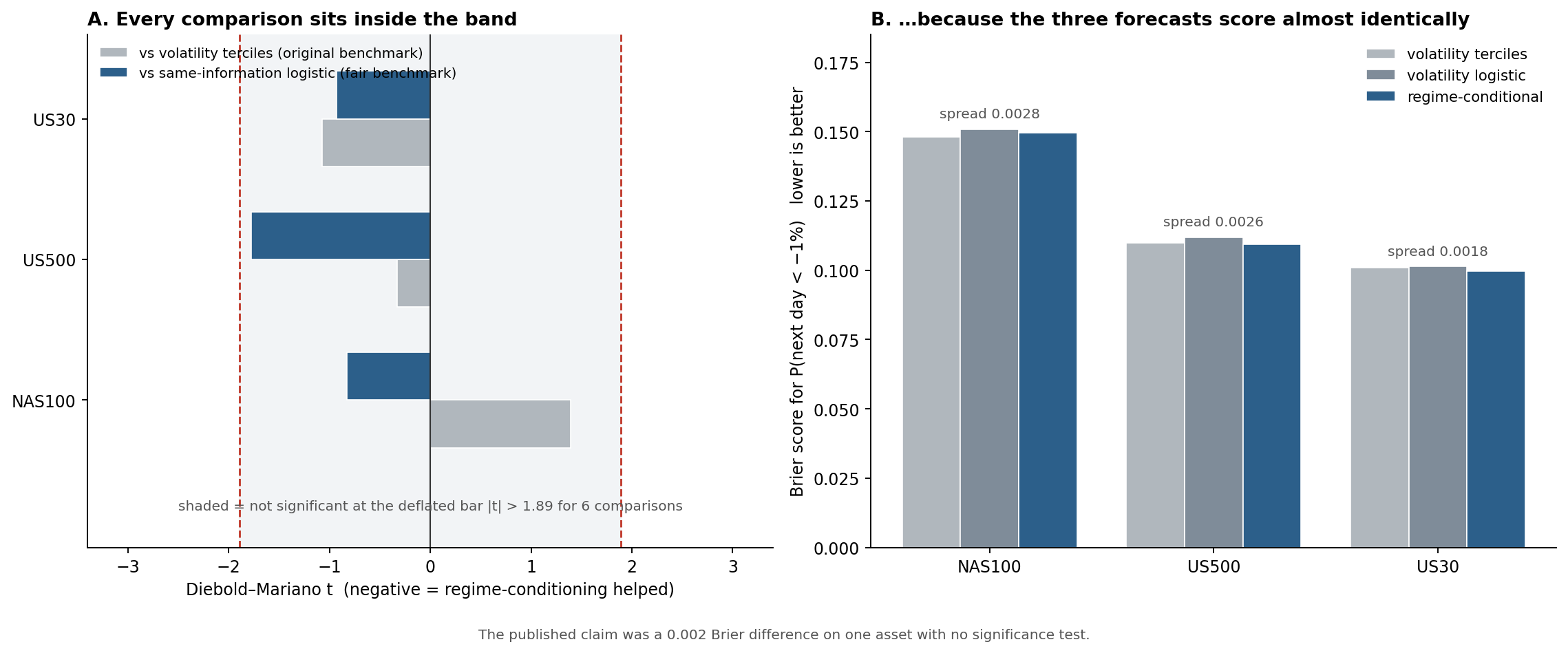
Nothing is significant. Zero of six comparisons clears the deflated bar of 1.89 — and zero clears even a naive 1.96:
| vs volatility terciles (original benchmark) | vs same-information logistic | |
|---|---|---|
| NAS100 | +0.0016 (t +1.39) | −0.0012 (t −0.83) |
| US500 | −0.0004 (t −0.33) | −0.0026 (t −1.78) |
| US30 | −0.0013 (t −1.07) | −0.0018 (t −0.93) |
On its own asset, against its own benchmark, the sign reverses. The claim was made on NAS100 against volatility terciles. Re-run with a proper test, the regime forecast there is worse than the tercile rule (+0.0016), not better. It is not significantly worse — but it is certainly not the published improvement.
Against a fair benchmark the direction is at least consistent. All three assets are negative against the same-information logistic, which is the same weak signature ewma_slope showed in RQ1: pointing the right way everywhere, reaching significance nowhere. Today has repeatedly shown that is not a finding.
The three forecasts are, for practical purposes, the same forecast. The total spread between terciles, logistic and regime is 0.0018 to 0.0028 Brier depending on the index. There is no room in that gap for a decision to change.
The verdict — H2 does not survive
The published claim — that regime-conditioning sharpens the probability of a dangerous day and beats a volatility benchmark — is not supported once the benchmark sees the same information and the difference is tested rather than asserted.
I do not think the original was carelessly computed. The numbers were right; the comparison was not. A 0.002 edge over a deliberately weaker benchmark is what a fair test is designed to catch, and it caught it.
This removes the proposal’s last untested positive. Every hypothesis that has now faced the full protocol — RQ1, RQ2/H1, H5 and H2 — has returned a null or a near-null. Only H6 (benefit concentrates at transitions) and H8 (hard risk limits improve viability) remain, and neither has been through it either. The proposal’s evidential position is weaker than the site claimed this morning, and saying so is the point of keeping a lab.
Limitations
- This is not an exact replication. The original used a two-state calm/turbulent HMM and an expanding-window event rate; this uses the harness’s three-state HMM on returns and a purged walk-forward logistic. It tests the same claim under the RQ1 protocol, not the same code. An exact re-run would need the original script, which was not kept.
- Three correlated indices. Six comparisons are not six independent tests, so the 1.89 bar is if anything lenient.
- Only the Brier claim is re-tested. The original also reported a large improvement in within-regime calibration error. That measure is not scored here, and a conditional- calibration advantage could exist even where the proper score shows nothing — though it would be a strange thing to build a proposal on, given a proper score is the thing that cannot be gamed.
- One target and one horizon. Next-day, −1%. The original’s two-sided robustness check is not repeated.
What I learned
The uncomfortable version: I found this by auditing which of my own results had been graded leniently, not by doubting the result itself. The tell was structural, not statistical — every surviving positive happened to predate the protocol. When the set of things you believe correlates that neatly with the set of things you tested least hard, the belief is about the testing, not the world.
The second lesson is that benchmark strength is a free parameter, and a quiet one. Nobody chooses a weak benchmark dishonestly; you choose the one that seems natural, and “event rate within a volatility bucket” seems perfectly natural until you notice the treatment is a filtered state-space model. Effect sizes are reported and scrutinised. Benchmark fidelity usually is not.
NAS100, US500, US30 daily from 2015 (--offline, committed CSVs); 1,780–1,810 scored days per asset. Target: next-day return < −1% (base rates 0.185, 0.128, 0.114). Forecasts: expanding event rate within trailing-volatility terciles; purged walk-forward logistic on [rv20, rv60]; the same logistic plus filtered hmm_gaussian state posteriors from the market-state-lab harness. All causal — the look-ahead guard applies to the state input. Scoring: Brier, Diebold-Mariano with Newey-West lag 1, deflated bar \sqrt{2\ln 6} = 1.89 over six comparisons. Significant results: 0 of 6. Brier spread across all three forecasts: 0.0028 (NAS100), 0.0026 (US500), 0.0018 (US30). Code in src/msl/metrics/calibration.py.