The AR Model (Autoregression)
Regressing a series on its own past — the one coefficient that separates mean reversion from a random walk
Autocorrelation measured how a series relates to its own past. The autoregressive model turns that measurement into a forecast: it regresses the series on its own lagged values, so the past becomes an explicit prediction of the present. One number — the AR(1) coefficient \phi — decides almost everything: whether the series mean-reverts, drifts as a random walk, or explodes. It is the model sitting underneath the two entries you just read, autocorrelation and stationarity, and the base that MA, ARIMA and GARCH build on.
The equation
An AR(1) regresses today on yesterday; the general AR(p) uses the last p values:
y_t = c + \phi\, y_{t-1} + \varepsilon_t \qquad\qquad y_t = c + \sum_{i=1}^{p}\phi_i\, y_{t-i} + \varepsilon_t
\varepsilon_t is white noise. For AR(1) the long-run mean is \mu = c/(1-\phi) and the autocorrelation function decays geometrically, \rho_k = \phi^{\,k}.
What each symbol means
| Symbol | Meaning |
|---|---|
| y_t | the series at time t |
| c | constant (intercept) — sets the long-run mean, c/(1-\phi) |
| \phi,\ \phi_i | the AR coefficient(s) — the weight on past values |
| y_{t-1} | the previous value (lag 1) |
| \varepsilon_t | white-noise shock (mean 0, constant variance) |
| p | the order — how many lags the model uses |
\phi is the memory dial: 0 means no memory, near 1 means long memory, exactly 1 is a random walk, and above 1 explodes.
Plain-English explanation
An autoregressive model says the next value is a scaled copy of the last one plus a fresh random shock. The scale factor \phi is the memory of the series. If \phi is 0 the past is irrelevant — pure white noise, every step a coin flip. If \phi is between 0 and 1 the series is pulled back toward its mean: a shock fades geometrically, and the closer \phi is to 1 the longer the memory. At \phi = 1 the pull vanishes entirely — shocks never fade and the series wanders with no home. That is a random walk, and it is exactly the unit root the ADF test hunts for. Push \phi above 1 and the series explodes.
So the whole behaviour of an AR(1) lives on a single dial. \phi = 0.9 means “mostly persistent but slowly reverting”; \phi = 1 means “random walk”; \phi = -0.5 means “overshoot and alternate.” The figure runs one set of random shocks through three values of \phi so you can watch the dial work.
Why it matters in markets
The AR coefficient is the bridge between the last three entries and the forecasting ones ahead, and its most important reading is the knife-edge at \phi = 1: below it the series is stationary and mean-reverting (worth modelling in levels); at it the series is a random walk (model the differences instead). That is no coincidence with the stationarity entry — the ADF regression is an AR model rearranged to test whether \phi = 1. And the AR(1) autocorrelation function \rho_k = \phi^{\,k} is exactly the geometric decay the autocorrelation entry drew: AR is the generative model behind that correlogram.
In markets the reading is sobering. Fit an AR(1) to index returns and \phi comes out near zero — the efficient-market result that returns barely predict themselves. Fit it to a price and \phi is essentially 1 — the random walk. The interesting cases are the constructed ones: a stationary spread (from cointegration), a volatility series, a rate — series with 0 < \phi < 1 and a finite mean-reversion half-life, \ln(0.5)/\ln(\phi), which is what pairs and mean-reversion strategies actually trade.
A simple worked example
Take AR(1) with c = 0.1, \phi = 0.6, starting at y_0 = 2, and ignore the shocks to see the pull. Each step multiplies the last value by 0.6 and adds 0.1: 2 \to 1.30 \to 0.88 \to 0.63 \to 0.48 \to 0.39, converging on the long-run mean \mu = c/(1-\phi) = 0.1/0.4 = 0.25. The gap to the mean shrinks by a factor 0.6 each step, so the half-life is \ln(0.5)/\ln(0.6) = 1.36 steps — after about 1.4 steps half of any shock is gone. That geometric pull toward a fixed level is the essence of a stationary AR process.
Python implementation
from statsmodels.tsa.ar_model import AutoReg
import numpy as np, pandas as pd

px = pd.read_csv("../multi_daily.csv", index_col="Date", parse_dates=True)["NDX"]
r  = px.pct_change().dropna()

fit    = AutoReg(r.values, lags=1, old_names=False).fit()   # AR(1) on returns
c, phi = fit.params                                          # -> phi = -0.121
half   = np.log(0.5) / np.log(abs(phi))                      # mean-reversion half-life
print(round(phi, 3), round(c, 5))                            # coefficient, constant
AutoReg(y, lags=p) fits AR(p) by OLS; .predict() forecasts. A \phi near 0 means the lag adds almost nothing — for returns, that is the whole story.
Manual / Excel calculation
AR(1) is a single regression of the series on its own one-step lag: put y_t in one column and y_{t-1} beside it (the same column shifted down a row), then:
| Task | Formula |
|---|---|
| \phi (AR-1 coefficient) | =SLOPE(B3:B1000, B2:B999) |
| c (constant) | =INTERCEPT(B3:B1000, B2:B999) |
| long-run mean | =c/(1-phi) |
| half-life | =LN(0.5)/LN(phi) |
For AR(p), regress on p lagged columns at once with LINEST.
Financial-market example — Nasdaq 100
The AR(1) coefficient tells the same story the earlier entries told, now compressed into one number:
| Series | AR(1) \phi | reading |
|---|---|---|
| NDX daily returns | −0.12 | barely predictable; mild one-day reversal |
| NDX price level | 1.00 | random walk — a unit root, non-stationary |
| NDX price − 200-day mean | 0.99 | mean-reverting, ~61-day half-life |
Fit to returns, \phi = -0.12 (t \approx -6.6): statistically real thanks to 2,900 observations, but tiny — the same faint one-day mean-reversion the autocorrelation entry measured, and far too small to beat costs. Fit to the price, \phi = 1.00: the textbook random walk, the unit root that made the price non-stationary. Neither is tradable as-is. The middle row is where AR earns its keep — the deviation of price from its 200-day mean has \phi \approx 0.99, a stationary series with a ~61-day half-life, the kind of mean-reverting construction (like a cointegrated spread) that mean-reversion strategies are built on.
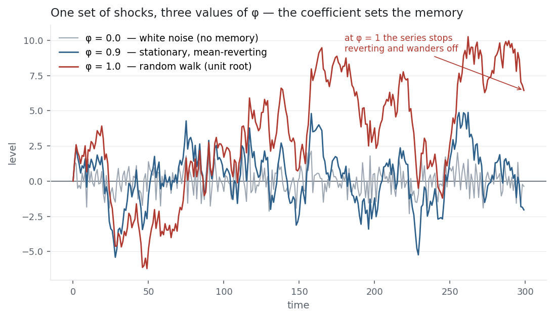
The three simulated paths share one set of shocks. At \phi = 0 the series is white noise; at \phi = 0.9 it takes long mean-reverting excursions; at \phi = 1 it stops reverting and wanders off. That last step — from 0.9 to 1.0 — is the entire difference between a stationary series you can model in levels and a random walk you must difference first.
Same multi_daily.csv as the previous entries (yfinance, adjusted closes); AR fits via statsmodels AutoReg. The three paths are simulated AR(1) processes sharing one set of shocks. Code blocks are illustrative — every number was computed and checked against the data.
Common mistakes
- Fitting AR to a non-stationary series in levels. If \phi \approx 1 the series has a unit root; model the differences (returns), not the level, or the estimates mislead.
- Reading a significant \phi as a tradable edge. The −0.12 on returns is real but tiny; statistical significance from a huge sample is not economic significance after costs.
- Confusing order p with fit quality. More lags fit the past better but overfit; pick p with AIC/BIC or the partial ACF, don’t just pile on lags.
- Forgetting \phi = 1 is the boundary. \phi just below 1 mean-reverts slowly; \phi = 1 never reverts. Tiny differences near the boundary change everything.
- Dropping the constant. The long-run mean is c/(1-\phi), not c; forcing no intercept forces mean zero.
- Expecting AR to capture volatility. AR models the level of returns (nearly unpredictable); the predictable part is the variance — that is what GARCH is for.