The Hurst Exponent
One number for memory — does a series trend, mean-revert, or wander at random?
This section has circled one question from every angle: does a series remember its past? Autocorrelation measured it lag by lag; AR and ARIMA modelled it; stationarity asked whether it wanders. The Hurst exponent answers the whole question with a single number. H sits between 0 and 1 and sorts every series into three worlds: below 0.5 it mean-reverts, at 0.5 it is a random walk, above 0.5 it trends. It is the natural finale for the time-series section — and applied to the Nasdaq it returns the same verdict everything else did.
The equation
The Hurst exponent H is defined by how the typical size of a move scales with the horizon. If \sigma(\tau) is the standard deviation of \tau-step changes,
\sigma(\tau) \propto \tau^{H}, \qquad H \in (0,1).
Equivalently, rescaled-range (R/S) analysis: over a window of length n, the rescaled range grows as
\mathbb{E}\!\left[\frac{R(n)}{S(n)}\right] \propto n^{H}.
H is the slope of \log(R/S) — or of \log \sigma(\tau) — against \log(\text{horizon}).
What each symbol means
| Symbol | Meaning |
|---|---|
| H | the Hurst exponent, in (0,1) |
| \tau,\ n | the horizon / window length |
| \sigma(\tau) | standard deviation of changes over horizon \tau |
| R(n) | the range (max − min of the cumulative deviations) over a window |
| S(n) | the standard deviation over that window |
| R/S | the rescaled range |
H = 0.5 is the random walk; H > 0.5 is persistent (trending); H < 0.5 is anti-persistent (mean-reverting).
Plain-English explanation
The Hurst exponent measures memory. Imagine watching how far a series drifts from its start as time passes. For a pure random walk, the distance grows like the square root of time — take four times as long and you get twice as far. That √time growth is H = 0.5, the fingerprint of no memory: each step is independent of the last.
H bends that scaling. If moves tend to continue — an up day breeds another up day — the series covers ground faster than √time, and H climbs above 0.5: it trends, it has positive long memory, it is “persistent.” If moves tend to reverse — up today, down tomorrow — the series covers ground slower than √time, and H falls below 0.5: it mean-reverts, “anti-persistent.” The further H is from 0.5, the stronger the memory; the closer, the more random. The figure shows the three textures: a high-H path is smooth and directional, a low-H path is jagged and self-cancelling, and H = 0.5 sits between.
Why it matters in markets
The Hurst exponent tells you which kind of strategy can possibly work, before you build one. In an H > 0.5 regime, momentum and trend-following have something to bite on — moves persist. In an H < 0.5 regime, mean-reversion strategies — pairs trades on a cointegrated spread, fading extremes — have the edge, because moves reverse. At H = 0.5 neither does: the series is a random walk and there is no memory to exploit. One number narrows the whole search.
It also ties this section back to the first: H = 0.5 is exactly the √time rule. That rule assumed volatility scales as \sqrt{\tau} — which is the statement that H = 0.5. So the Hurst exponent is the parameter the √time rule quietly fixed at one-half; measuring H \ne 0.5 is measuring the precise way real returns violate it. A trending market’s volatility grows faster than √time (H > 0.5); a mean-reverting one’s grows slower (H < 0.5). Persistence, mean reversion, and the annualisation rule are three faces of the same exponent.
A simple worked example
Suppose a series moves with a typical daily change of 1%. Over 9 days, how far does it drift? For a random walk (H = 0.5) the answer is the √time rule: 1\% \times 9^{0.5} = 3\%. If the series trends (H = 0.7): 1\% \times 9^{0.7} = 4.7\% — persistence compounds the moves, so it travels farther. If it mean-reverts (H = 0.3): 1\% \times 9^{0.3} = 1.9\% — reversion cancels moves, so it stays closer to home. Same daily volatility, three different multi-day risks, set entirely by H. That single exponent is why “scale by √time” is right only for a random walk.
Python implementation
import numpy as np, pandas as pd

lp = np.log(pd.read_csv("../multi_daily.csv", index_col="Date", parse_dates=True)["NDX"])

def hurst(series, lags=range(2, 200)):
    s   = np.asarray(series, float)
    tau = [np.std(s[L:] - s[:-L]) for L in lags]              # std of L-lag changes
    return np.polyfit(np.log(list(lags)), np.log(tau), 1)[0]  # slope = H

print(round(hurst(lp.values), 3))      # -> 0.434   (variance-scaling estimate)
Estimators disagree at the edges (R/S, DFA, variance-scaling); report the method and a sanity check — a synthetic random walk should read ≈ 0.5.
Manual / Excel calculation
The variance-scaling recipe is spreadsheet-friendly: for each lag \tau, compute the standard deviation of the \tau-step changes (=STDEV of the differenced series), then regress log(σ) on log(τ) with =SLOPE(LN(sigmas), LN(taus)). That slope is H. The classic R/S method is fiddlier by hand (cumulative deviations, range over standard deviation, across many window sizes) — use a package for it.
Financial-market example — Nasdaq 100
Estimate H on eleven years of NDX log price and the verdict matches the whole section: H \approx 0.43 by variance-scaling (stable across lag windows, 0.42 to 0.46) and \approx 0.51 by rescaled-range — both hugging the 0.5 random-walk line. The small shortfall below 0.5 is mostly estimator bias: the same variance-scaling method reads a synthetic random walk at 0.47, not 0.50. So the honest read is H \approx 0.5 — the Nasdaq is a random walk, with at most a faint mean-reverting lean, the same whisper that showed up as the −0.12 lag-1 autocorrelation and is just as untradable.
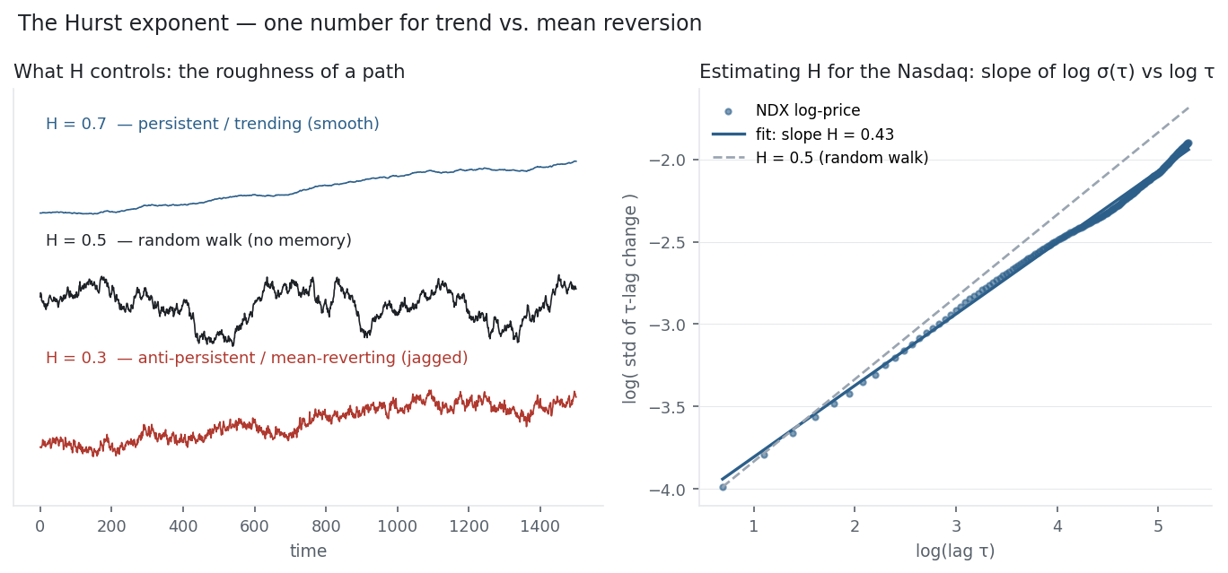
The right panel is the estimate: NDX’s log σ(τ)-vs-log τ points fall almost exactly on the H = 0.5 reference, a hair shallower. The left panel is the point of the whole exercise — a trending H = 0.7 world and a mean-reverting H = 0.3 world look nothing alike, and identifying which one you are in is the first question any strategy should ask. For the Nasdaq index the answer is “neither” — but for a cointegrated spread it would be H < 0.5, and that is where the mean-reversion trades of this section live.
Same multi_daily.csv as the previous entries (yfinance, adjusted closes). H by variance-scaling on log price, cross-checked with R/S; the three example paths are simulated fractional Brownian motions. Every number was computed and checked.
Common mistakes
- Reading H as constant. It shifts with regime and horizon; a market can trend intraday and mean-revert weekly. Estimate it on the horizon you trade.
- Trusting one estimator. R/S, DFA and variance-scaling can disagree by 0.05+; cross-check and bias-test against a synthetic random walk.
- Over-interpreting H near 0.5. Tiny deviations (0.47 vs 0.50) are usually estimation noise, not signal — as with NDX.
- Confusing persistence with predictable return. H > 0.5 means moves persist statistically, not that the next move is a sure thing or survives costs.
- Applying it to too little data. R/S and variance-scaling need long series; short samples give wildly unstable H.
- Running it on the wrong series. Hurst on a price (levels) answers trend/reversion; on stationary returns it collapses toward 0 — pick the series that matches the question.