Convolutional Neural Networks

Weight sharing and local filters — the architecture that put a prior into the network

A CNN slides small shared filters across grid-structured data to detect local, translation-invariant patterns at a fraction of a dense net’s parameters. Convolution, pooling, the inductive bias, and an honest 1D-CNN test on Nasdaq sequences.

The multilayer perceptron connected every input to every neuron — it assumed nothing about how the inputs relate to each other. A convolutional neural network is the first architecture on this site to build in a prior: it assumes the useful patterns are local (a small neighbourhood is enough) and translation-invariant (the same pattern means the same thing wherever it appears), and it encodes that assumption directly by sliding a small, shared filter across the input. For images — where an edge is an edge in any corner of the frame — this prior is exactly right, and it is what made deep learning work on vision. The question for a quant is whether a price or return sequence has the same kind of structure. It partly does, and partly doesn’t, in the way that by now you can probably guess.

1. What problem does it solve?

Supervised learning on grid-structured data with local, repeatable patterns — 2D images, 1D sequences and audio, 3D volumes — where a feature (an edge, a texture, a motif) carries the same meaning regardless of where it occurs. A CNN learns a hierarchy of local feature detectors: early layers pick up simple patterns, later layers combine them into complex ones. It is the workhorse of computer vision; in a quant context, a 1D CNN is a learnable pattern detector over a time series.

2. What assumptions does it make?

Its whole identity is an inductive bias: that useful features are local (a small window suffices to detect them), translation-invariant (position doesn’t change their meaning), and compositional (complex patterns are combinations of simpler ones). These priors are almost perfectly true for natural images. For financial sequences they are a bet that predictive local motifs exist — a bet that, as the market test shows, pays off for volatility structure and fails for direction. Crucially, a CNN assumes the input axis has real locality: neighbouring points are related. Shuffle the columns of the input and a CNN breaks while a dense net wouldn’t — the ordering is the assumption.

3. What data does it need?

Data on a grid whose axes carry meaning: pixels laid out in space, returns laid out in time. Because it shares weights, a CNN is dramatically more parameter-efficient than a dense net on the same grid, so it needs less data to generalise — the built-in prior does work that data would otherwise have to. It benefits from scale like any deep model, but its efficiency is exactly why it can succeed on modest datasets where a dense net of equal reach would overfit.

4. How does it work?

The core operation is the convolution. A small filter (kernel) of shared weights slides across the input, computing a dot product at each position to produce a feature map — a signal that lights up wherever the filter’s pattern occurs. A width-3 filter of [1,1,1]/3 is a moving average (a smoother); [-1,0,1] is a momentum/slope detector; a filter tuned to a burst fires at a volatility cluster. A layer applies many filters, each learning a different pattern, giving many feature maps. Three properties define it:

• Weight sharing. The same filter is reused at every position. To map a length-20 input to 18 outputs, a dense layer needs 20\times18 = 360 weights; a width-3 convolution needs 3 — 120× fewer — because those three weights are shared across all positions. A realistic 16-filter conv layer uses 64 parameters where the equivalent dense layer needs over 6,000.
• Local receptive fields. Each output depends only on a small input window, matching the locality assumption.
• Translation equivariance. Because the filter is shared, a pattern shifted along the input produces the same response, shifted — the left panel shows one filter detecting the identical burst at two different positions.

After the convolution comes a nonlinearity (ReLU) and usually pooling, which downsamples each feature map (taking the max or average over small windows) — shrinking the representation and converting equivariance into invariance (the pattern is detected whether or not it moves a little). Stacking convolution–ReLU–pool blocks builds the hierarchy: edges → textures → shapes. The filters themselves are just weights, learned end-to-end by backpropagation exactly like any other network.

5. What are its strengths?

• Parameter efficiency. Weight sharing slashes the parameter count, cutting both memory and overfitting — often an order of magnitude fewer weights than a dense net for the same input.
• Translation invariance. A pattern is detected wherever it appears, learned once and reused everywhere.
• Hierarchical feature learning. Simple local features compose into complex ones automatically, with no hand-engineering.
• The right prior for grid data. On images and other local-structured signals its inductive bias is correct, which is why it dominates computer vision.
• Fast. Convolutions are cheap and massively parallelisable on modern hardware.

6. What are its weaknesses?

• The prior can be wrong. If structure isn’t local or translation-invariant — non-grid data, or long-range dependencies — the assumption hurts more than it helps.
• Limited receptive field. Each layer sees only a small window; capturing long-range relationships needs depth, dilation, or a different architecture.
• Not built for order-sensitive sequences. For variable-length or strongly sequential data, RNNs and transformers model dependencies more naturally.
• Still a black box. Learned filters are more interpretable than a dense net’s weights, but a deep stack remains opaque.
• No help where there’s no local signal. On markets it detects the motifs that exist and, like everything here, invents none that don’t.

7. How could it apply to markets?

A 1D CNN treats a window of history as a sequence and learns filters that fire on local patterns — momentum bursts, volatility clusters, reversal shapes. To test it honestly I trained a small one (8 filters, width 3, global pooling — just 41 parameters) on the same tasks as every other model here.

Left: one width-3 filter slid across a sequence detects the same “burst” motif at two different positions — local, translation-invariant pattern detection with just 3 shared weights, where a dense layer would need 360. Right: a 1D CNN on Nasdaq sequences reaches 0.57 test AUC on volatility — matching a dense MLP that uses 5× as many parameters (193 vs 41) — but only 0.49 on direction, a coin flip.

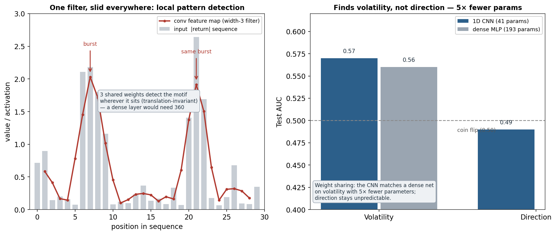
The result is the cleanest illustration yet of what an inductive bias can and can’t do. On predicting a high-volatility day the CNN scores a test AUC of 0.57 — right in line with the random forest, boosting, the SVM, and the dense net — and it gets there with 41 parameters against the dense net’s 193, a 5× saving from weight sharing at equal accuracy. This makes sense: a convolutional filter that responds to a cluster of large recent moves is a volatility-burst detector, and volatility clustering is a genuinely local, repeatable motif, so the CNN’s prior fits it perfectly. On predicting direction the same architecture manages AUC 0.49 — a coin flip — because there is no repeatable local motif in signed returns that foretells the next day. The architecture is more elegant and far more efficient, and it reaches the identical verdict: the inductive bias earns its keep where local structure exists (volatility) and cannot manufacture signal where it doesn’t (direction). Where a CNN would genuinely shine is on truly spatial market data — a limit-order book snapshot treated as an image — not a plain vector of lagged returns.

8. What does the Python code look like?

import torch.nn as nn

# a 1D CNN over a length-L window of returns (1 input channel)
model = nn.Sequential(
    nn.Conv1d(in_channels=1, out_channels=8, kernel_size=3),   # 8 filters, width 3 -> 8*3+8 = 32 params
    nn.ReLU(),
    nn.AdaptiveAvgPool1d(1),                                    # global pooling -> one value per filter
    nn.Flatten(),
    nn.Linear(8, 1))                                            # + 9 params  ->  ~41 total
# vs a Linear(20, 16) first layer alone = 336 params: weight sharing is the saving

out_channels is the number of pattern detectors; kernel_size is the window; the parameter count is out_channels × kernel_size regardless of input length — that length-independence is weight sharing. Pooling gives translation invariance and shrinks the representation.

9. How would I explain it to a supervisor?

“A CNN is a neural network with a built-in assumption: that useful patterns are local and mean the same thing wherever they appear. So instead of connecting everything to everything, it slides a small shared filter across the input to build a feature map, uses many filters to detect many patterns, and pools to gain translation invariance — all trained by backprop. Weight sharing makes it hugely parameter-efficient: a width-3 filter uses 3 weights where a dense layer would use hundreds. On the Nasdaq I trained a 41-parameter 1D CNN and it hit 0.57 AUC on volatility — matching a dense net with five times the parameters, because a convolution is a natural volatility-burst detector — but 0.49 on direction, a coin flip. The right prior for local structure, efficient and elegant, and it confirms the same thing: volatility has local structure, direction doesn’t. On genuinely spatial market data like an order-book image it would have a real edge.”

1D CNN (8 width-3 filters, ReLU, global-average pooling, linear output — 41 parameters) implemented and trained by hand in NumPy, on the same Nasdaq multi_daily.csv tasks and 70/30 time split as the earlier models; standardised inputs. Volatility/direction AUCs, the dense-MLP comparison (193 parameters), and the weight-sharing parameter counts were computed and checked.