Decision Trees

A flowchart of if-then splits — nonlinear, interpretable, and prone to overfitting

Decision trees recursively split feature space to cut impurity (Gini/entropy). Nonparametric and interpretable, they capture nonlinearities — but a single tree overfits, memorising the Nasdaq’s noise while generalising to the base rate.

Decision trees are the first nonlinear model in this library — and the first that can’t be written as a single equation. A tree is a flowchart of yes/no questions (“is today’s return above 0.5%? is momentum below −2%?”) that splits the data into ever-smaller groups, and predicts the majority class (or average value) in each final group. It carves feature space into rectangles where the linear models could only draw a line, and it does so by the exact impurity measures from the Equation Library — Gini and entropy / information gain. Its gift is interpretability; its curse is that, left alone, it overfits almost anything.

1. What problem does it solve?

Both classification and regression, by recursively partitioning the feature space into homogeneous regions. Each internal node is a threshold test on one feature; each leaf is a prediction — the majority class, or the mean target, of the training points that land there. The whole model is a readable set of if-then rules, which is much of its appeal.

2. What assumptions does it make?

Almost none — it is nonparametric. It assumes nothing about the distribution of the features, needs no linearity, and requires no scaling (splits are threshold comparisons, invariant to monotonic transforms). Its one structural assumption is that the target can be approximated by axis-aligned, piecewise-constant regions — so it captures interactions and non-monotonic effects easily, but represents a diagonal boundary only as a clumsy staircase of rectangles.

3. What data does it need?

Features (numeric or categorical, unscaled) and a target. It handles mixed types, non-linear relationships, and interactions natively, and some implementations handle missing values. What it needs above all is enough data per leaf: because it keeps splitting until groups are pure, a small dataset lets it carve one leaf per noisy point — the root of its overfitting.

4. How does it learn?

Greedily, by recursive partitioning (the CART algorithm). At each node it searches every feature and threshold for the split that most reduces impurity — Gini or entropy for classification (the drop is the information gain), or variance / MSE for regression — takes the best one, and recurses on each child until a stopping rule (max depth, minimum samples per leaf, or a pure node) halts it. It is greedy, not globally optimal: it never reconsiders an earlier split. Growing it fully and then pruning back, or capping depth and leaf size up front, is how you regularise it — the complexity control that decides whether it generalises or memorises.

5. What are its strengths?

• Interpretable. The model is a flowchart; you can read the rules and explain any prediction.
• Nonlinear and interaction-aware for free. No feature engineering needed to capture curves or “A only matters when B is high.”
• No preprocessing. No scaling, no encoding of ordinals; robust to monotonic transforms and outliers in the features.
• Mixed data and fast prediction. Handles numeric and categorical together; a prediction is a handful of comparisons.
• Feature importance. Reports which features drove the most impurity reduction.

6. What are its weaknesses?

• High variance — it overfits. A deep tree fits every wiggle of the training data; small data changes produce a completely different tree.
• Greedy, not optimal. Each split is chosen locally; the tree can miss a better global structure.
• Axis-aligned only. Diagonal or smooth boundaries need many staircase splits, which overfit.
• Biased to high-cardinality features. Raw impurity gain favours features with many split points (the information-gain bias).
• A single tree is rarely the final model. Its variance is why practitioners almost always ensemble trees — into random forests and gradient boosting (the next entries).

7. How could it apply to markets?

The appealing use is interpretable, rule-based signals: “if the VIX is above 25 and 5-day momentum is negative, expect turbulence” is a decision tree, and its transparency is valuable when a supervisor or risk committee needs to see the logic. Trees also handle the interactions and regime effects that linear models miss. But on noisy financial data a single tree is a cautionary tale, not a solution — it will find “rules” in pure chance.

Left: as tree depth grows, training accuracy climbs toward 100% (it memorises the training days) while out-of-sample accuracy stays flat at the ~57% base rate — the signature of overfitting. Right: a depth-5 tree’s decision regions on two features — axis-aligned rectangles (blue predicts up, red down), a patchwork fitted to noise rather than a real boundary.

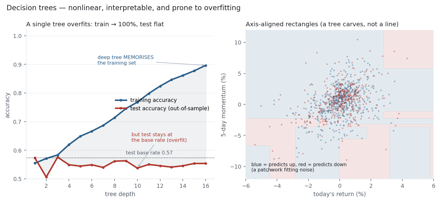
The figure is the honest lesson. Trained to predict the Nasdaq’s next-day direction from its last 20 returns, a shallow tree does nothing (train and test both near the base rate), but as you let it grow, the training accuracy marches from 56% to 100% — a fully grown tree (depth 27) classifies every training day correctly. Its test accuracy, meanwhile, never leaves the base rate and actually dips below it. The tree isn’t learning the market; it is memorising the training set’s noise, one leaf at a time. The right panel shows the same thing spatially: the up- and down-days overlap entirely, and the tree responds by chopping the plane into a meaningless patchwork of rectangles. A single decision tree, on a near-efficient market, is overfitting made visible.

8. What does the Python code look like?

from sklearn.tree import DecisionTreeClassifier
from sklearn.metrics import accuracy_score

# depth is the main regularisation knob:
tree = DecisionTreeClassifier(max_depth=3, min_samples_leaf=50).fit(X_train, y_train)
print(accuracy_score(y_test, tree.predict(X_test)))       # shallow: ~ base rate, honest

full = DecisionTreeClassifier().fit(X_train, y_train)      # unlimited depth
print(accuracy_score(y_train, full.predict(X_train)))      # -> 1.00  (memorised)
print(accuracy_score(y_test,  full.predict(X_test)))       # -> ~0.54 (base rate)
# tree.feature_importances_  and  sklearn.tree.plot_tree() to read the rules

criterion="gini" (default) or "entropy" chooses the impurity measure — they give nearly identical trees. Cap max_depth / min_samples_leaf or prune (ccp_alpha) to control overfitting.

9. How would I explain it to a supervisor?

“A decision tree is a flowchart of if-then splits, each chosen to reduce impurity — Gini or entropy for classification, variance for regression — grown greedily and pruned back to control complexity. It’s nonparametric, needs no scaling, captures interactions, and is fully interpretable, which is its main advantage. Its weakness is high variance: on the Nasdaq a full tree hits 100% training accuracy but generalises only to the base rate, textbook overfitting. That variance is exactly why we don’t use single trees in practice — we average many of them in a random forest, or boost them, which is where I’d go next.”

Nasdaq-100 basket from the same multi_daily.csv as the Equation Library (yfinance, adjusted closes). Train/test accuracy vs depth on 20 lagged returns (70/30 time split), the fully-grown-tree figures, and the two-feature decision boundary were all computed and checked.