EGARCH, GJR & HAR-RV — Asymmetric and Realized Volatility
Two things vanilla GARCH misses: the leverage effect (down moves raise vol more) and the forecasting power of a realized measure
The GARCH entry established that volatility clusters and is forecastable — the one genuinely predictable thing on this site. But plain GARCH is symmetric (it treats a crash and a rally of equal size identically) and returns-based (it learns from squared returns, not from a direct measurement of variance). Both are limitations a real volatility specialist fixes. EGARCH and GJR-GARCH add the leverage effect — the robust fact that markets get more volatile after falling than after rising. HAR-RV forecasts volatility from a realized measure across heterogeneous horizons, and does it with an ordinary regression. This entry builds all three, and they are exactly the tools the proposal’s Volatility specialist should carry.
1. What problem does it solve?
Making the volatility model match two facts that plain GARCH ignores. First, asymmetry: a −3% day and a +3% day do not imply the same tomorrow — fear, deleveraging and margin calls make downside shocks raise volatility more. A symmetric model is mis-specified against one of the most robust stylised facts in finance. Second, the measure: squared daily returns are a noisy proxy for a day’s true variance, and models fit to a realized measure (built from intraday data, or here from the daily range) forecast better. EGARCH/GJR solve the first; HAR-RV solves the second. Together they turn “volatility is forecastable” into “here is the forecast, with the leverage effect and horizon structure built in.”
2. The leverage effect, and two ways to model it
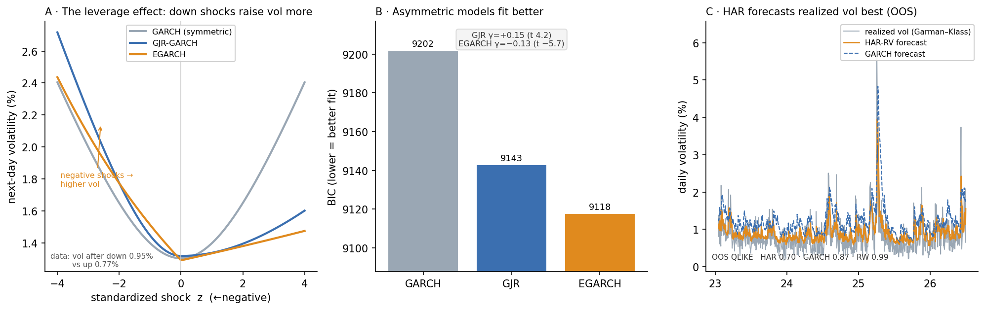
The asymmetry is visible before any model. On the Nasdaq, the average next-day realized volatility is 0.95% after down days versus 0.77% after up days — a 24% difference conditioned only on the sign of today’s return. Two standard models capture it. GJR-GARCH adds an extra ARCH term that only fires on negative shocks:
\sigma_t^2=\omega+\alpha\,\varepsilon_{t-1}^2+\gamma\,\varepsilon_{t-1}^2\,\mathbf{1}\{\varepsilon_{t-1}<0\}+\beta\,\sigma_{t-1}^2,
so a positive \gamma means downside shocks add more variance. EGARCH models the log variance — which needs no positivity constraints — and puts the asymmetry in a signed term:
\ln\sigma_t^2=\omega+\beta\ln\sigma_{t-1}^2+\alpha\big(|z_{t-1}|-\mathbb{E}|z|\big)+\gamma\,z_{t-1},\qquad z_t=\varepsilon_t/\sigma_t,
where a negative \gamma makes negative standardized shocks raise volatility more. Fit to Nasdaq returns, both find the asymmetry strongly significant — GJR \gamma=+0.154 (t=4.2), EGARCH \gamma=-0.126 (t=-5.7) — and both beat symmetric GARCH decisively on BIC (9202 → 9143 → 9118), EGARCH best. Persistence is essentially unchanged (GARCH 0.975, GJR 0.967, EGARCH \beta 0.957), so the asymmetric term is adding a genuinely new feature — direction-dependence — not just re-describing the clustering the GARCH entry already measured. The news-impact curve (left panel) makes it visual: the same shock maps to a higher next-day volatility when it is negative.
3. HAR-RV — forecasting from a realized measure across horizons
Corsi’s Heterogeneous Autoregressive model forecasts tomorrow’s realized variance as a simple linear combination of daily, weekly and monthly realized variance — a nod to the idea that traders operate on different horizons, and a way to mimic long memory with three regressors:
RV_{t+1}=\beta_0+\beta_d\,RV_t^{(d)}+\beta_w\,RV_t^{(w)}+\beta_m\,RV_t^{(m)}+\varepsilon_{t+1}.
The realized measure matters. Rather than squared close-to-close returns, I use the Garman-Klass estimator, which uses the full daily range (O,H,L,C) and is several times more efficient: \widehat\sigma^2_t=\tfrac12(\ln H_t/L_t)^2-(2\ln 2-1)(\ln C_t/O_t)^2. Fit on 2015–2022 and tested on 2023–2026, HAR puts most weight on the weekly term (coefficients: daily 0.27, weekly 0.49, monthly 0.02) and forecasts next-day volatility better than the alternatives on every metric:
| Model (1-day-ahead) | QLIKE | RMSE (vol) | R² (var) |
|---|---|---|---|
| Random walk (yesterday’s RV) | 0.995 | 0.447 | 0.062 |
| GARCH(1,1) | 0.868 | 0.613 | −0.440 |
| HAR-RV | 0.702 | 0.397 | 0.255 |
The honest reading of that table is a lesson in itself. HAR wins because it is fit directly on the realized measure it is scored against — Corsi’s whole point. GARCH is competitive on QLIKE (0.87, well below the random walk) but has a negative R², because it is a returns-based model asked to predict a range-based target: its forecasts are the right shape but the wrong scale, sitting systematically high (the blue dashed line in the right panel). This is not GARCH failing at what it does — it is the practical case for realized-measure models when the quantity you actually care about is a realized measure. It also sharpens the Quant-Lab horizon experiment, which found GARCH and HAR close on QLIKE when both target squared returns: against a range-based realized measure, HAR’s direct-fit advantage widens.
4. What are its strengths?
- The leverage effect is real and cheap to add. One extra parameter turns a mis-specified symmetric model into one that respects the most robust asymmetry in equity volatility, with strong statistical support (BIC, significant \gamma).
- EGARCH needs no constraints. Modelling log-variance means the variance is positive automatically, so estimation is stable and the asymmetry term is unrestricted.
- HAR is absurdly simple and hard to beat. An OLS regression on three horizons forecasts volatility as well as or better than parametric GARCH — the workhorse of the realized-volatility literature for good reason.
- Realized measures beat squared returns. Using the daily range (Garman-Klass) rather than close-to-close squared returns injects a far more efficient measurement, and HAR exploits it directly.
- Horizon structure is explicit. HAR’s daily/weekly/monthly decomposition is interpretable and maps onto the multi-horizon view the proposal takes of the market.
5. What are its weaknesses?
- Asymmetry is fit, not alpha. A better-fitting variance model is honesty about risk, not a return signal — it tells you when volatility will be high, which the site shows is the forecastable part, not which way prices go.
- Measure mismatch cuts both ways. HAR’s win partly reflects being scored on the measure it was fit to; a model must be evaluated on the quantity you actually use, and swapping the realized proxy can move the ranking.
- Daily data limits the “realized” measure. True HAR uses intraday realized variance; with daily OHLC I use a range estimator, which is a legitimate but coarser proxy — the high-frequency version would do better still.
- Still Gaussian-ish and linear. EGARCH/GJR assume a parametric innovation and HAR is linear in its regressors; jumps, fat tails and structural breaks are only partially handled.
- Parameters drift. Volatility dynamics are themselves non-stationary; a single fitted model will decay, which is why these feed a system with change-point and regime machinery around them.
6. How could it apply to markets?
In the proposal these are the Volatility specialist’s core estimators, and the results dictate its design. It should be asymmetric — the leverage effect is too significant to ignore, so a GJR or EGARCH conditional variance, not a symmetric GARCH, drives the “expansion probability” the specialist emits. It should be realized-measure-based — HAR on a range or intraday measure is the best one-day-ahead forecaster here, so it, not squared-return GARCH, produces the point forecast, with its daily/weekly/monthly structure giving the expected-horizon field directly. And the specialist’s output must be honest about the measure: the negative-R² lesson is that a forecast is only as good as its match to the quantity a downstream agent consumes, so the volatility evidence is emitted with its definition attached. These estimators also feed the rest of the site: the leverage effect is why the volatility-managed strategy cuts exposure into falling, volatile markets, and the conditional variance is the \sigma_t that makes conformal intervals and risk limits regime-honest. Volatility is the one thing markets let you forecast; these are the models that forecast it properly.
7. What does the Python code look like?
import numpy as np, pandas as pd
from arch import arch_model                      # GARCH / GJR / EGARCH by MLE

r = 100 * np.diff(np.log(close))                 # % log returns
garch = arch_model(r, vol="GARCH", p=1,      q=1).fit(disp="off")   # symmetric
gjr   = arch_model(r, vol="GARCH", p=1, o=1, q=1).fit(disp="off")   # o=1 -> leverage term
egarch= arch_model(r, vol="EGARCH",p=1, o=1, q=1).fit(disp="off")   # log-variance, asymmetric
# asymmetry parameter gamma and its t-stat decide whether the leverage effect is real:
print(gjr.params["gamma[1]"], gjr.params["gamma[1]"] / gjr.std_err["gamma[1]"])

# HAR-RV on a Garman-Klass realized measure (uses the daily range, not just the close)
gk = 0.5*(np.log(H/L))**2 - (2*np.log(2)-1)*(np.log(C/O))**2        # daily realized variance
RV = pd.Series(gk)
X  = np.column_stack([np.ones(len(RV)), RV, RV.rolling(5).mean(), RV.rolling(22).mean()])
y  = RV.shift(-1).values                                            # predict next-day RV
b  = np.linalg.lstsq(X[ok_train], y[ok_train], rcond=None)[0]       # daily / weekly / monthly betas
har_forecast = X @ b
Three parametric models and one three-line regression — and the regression is the one that forecasts best.
8. How would I explain it to a supervisor?
“Plain GARCH misses two things a volatility desk cares about, so I added the models that fix them. First, the leverage effect: Nasdaq volatility is higher after down days than up days — 0.95% versus 0.77% — and GJR-GARCH and EGARCH both capture that asymmetry with a strongly significant parameter, t-stats of about 4 and −6, and both beat symmetric GARCH on BIC. Persistence barely changes, so the asymmetry is a genuinely new feature, not a re-description of clustering. Second, the measure: I built HAR-RV, Corsi’s regression of tomorrow’s realized variance on daily, weekly and monthly realized variance, using a Garman-Klass range estimator instead of squared returns. Out of sample it forecasts next-day volatility better than GARCH or a random walk on QLIKE — 0.70 versus 0.87 versus 0.99 — because it’s fit directly on the realized measure. There’s an honest subtlety: GARCH has a negative R² against that target because it’s a returns-based model predicting a range-based measure, so it’s the right shape but the wrong scale — which is exactly the argument for realized-measure models when a realized measure is what you’ll use. For my proposal, the Volatility specialist should therefore be asymmetric and realized-measure-based, and it should always emit its volatility estimate with the measure it was fit to attached.”
Data: NDX daily OHLC 2015–2026 (2,892 returns). Models fit with arch 8.0. GARCH(1,1) loglik −4585.1, BIC 9202.0, α 0.131, β 0.844, persistence 0.975. GJR-GARCH loglik −4551.6, BIC 9143.0, α 0.027, γ +0.154 (t 4.15), β 0.863, persistence 0.967. EGARCH(1,1) loglik −4539.0, BIC 9117.8, α 0.192, γ −0.126 (t −5.65), β 0.957. Model-free leverage: mean next-day Garman-Klass realized vol 0.95% after down days vs 0.77% after up (ratio 1.24). HAR-RV on Garman-Klass realized variance, train 2015–2022 / test 2023–2026, coefficients const 0.239, daily 0.269, weekly 0.493, monthly 0.020. Out-of-sample (next-day realized variance): QLIKE random walk 0.995 / GARCH 0.868 / HAR 0.702; RMSE(vol) 0.447 / 0.613 / 0.397; R²(var) 0.062 / −0.440 / 0.255. GARCH OOS forecast is a fixed-parameter one-step recursion; QLIKE =\overline{RV/h+\ln h}. Every number was checked.