Logistic Regression

A probability from a linear score — the classification baseline

Logistic regression squashes a linear score through the sigmoid into a probability, trained by cross-entropy. Log-odds interpretability, the linear decision boundary, and an honest Nasdaq direction test (AUC ≈ 0.51).

Logistic regression is linear regression’s classifier cousin: it takes the same linear score w\cdot x + b and, instead of using it as a prediction, squashes it through the sigmoid into a probability between 0 and 1. Train it by minimising cross-entropy and you have the workhorse baseline for classification — interpretable, fast, and probabilistic. The name is a historical quirk (it does classification, not regression), but the machinery is exactly the maths from the Equation Library, assembled into a model.

1. What problem does it solve?

Binary (and, via softmax, multi-class) classification: output the probability that an example belongs to a class, \hat p = \sigma(w\cdot x + b), then threshold it (usually at 0.5) for a hard label. It answers “how likely is this to be class 1, given the features?” — and, because it is a probability, it also says how confident the model is.

2. What assumptions does it make?

That the log-odds are linear in the features: \ln\frac{p}{1-p} = w\cdot x + b. That gives a straight-line (hyperplane) decision boundary. It also assumes independent observations and no perfect multicollinearity. Notably it does not assume the features are normally distributed or have equal variance — the assumptions are on the boundary’s shape, not the inputs’ distribution. The one thing it hates is perfect separation: if a feature splits the classes cleanly, the optimal weights run to infinity, which is why regularisation is standard.

3. What data does it need?

Features and a binary (or categorical) target; enough examples of each class; features scaled if you will regularise or compare coefficients. Categorical inputs must be encoded. It tolerates correlated and non-normal features, but a genuinely linear separation in log-odds space has to roughly exist for it to classify well.

4. How does it learn?

It computes a probability \hat p = \sigma(w\cdot x + b) and minimises the cross-entropy loss between those probabilities and the true labels. Unlike linear regression there is no closed form — the loss is minimised by gradient descent, and here the maths is especially clean: the gradient of cross-entropy through the sigmoid is exactly (\hat p - y), predicted minus actual, the same cancellation that made softmax + cross-entropy universal. Each coefficient w_j is the change in log-odds per unit of feature j, so e^{w_j} is an odds ratio — a w_j of 0.7 means a one-unit rise roughly doubles the odds (e^{0.7} = 2.0).

5. What are its strengths?

• Probabilistic and calibrated. It outputs a genuine probability, not just a label — essential for sizing bets or ranking risk.
• Interpretable. Coefficients are log-odds effects; e^{w} is an odds ratio a supervisor or regulator can read.
• Fast and convex. The cross-entropy loss is convex, so gradient descent finds the global optimum; no tuning drama.
• A strong linear baseline. The classification counterpart of linear regression — what every fancier classifier must beat.
• Regularisable. L1/L2 penalties plug straight in for selection and stability.

6. What are its weaknesses?

• Linear boundary only. It can only separate classes with a hyperplane; curved boundaries need engineered features or a different model.
• Fragile under separation. Perfectly separable classes send the weights to infinity — regularisation or early stopping is required.
• Outlier- and scale-sensitive. Extreme feature values distort the boundary; standardise inputs.
• Assumes log-odds linearity. If the true relationship is non-monotonic, the fit is biased.
• Not a probability oracle. Well-calibrated only if the linear-in-log-odds assumption roughly holds; check calibration.

7. How could it apply to markets?

The obvious use is direction: classify tomorrow as up or down from today’s features. It is also the standard tool for credit default probability, regime classification (calm vs. turbulent), and any “will this event happen?” question where a calibrated probability beats a yes/no. The catch, as ever, is that predicting the direction of a liquid index is close to hopeless — and logistic regression, being honest and probabilistic, shows exactly how hopeless.

Left: next-day up (blue) vs down (red) days plotted against today’s return and 5-day momentum — the classes overlap completely, so the linear boundary can’t separate them. Right: the out-of-sample ROC curve sits on the random diagonal (test AUC ≈ 0.51).

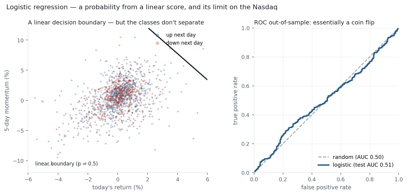
Fit logistic regression to predict the Nasdaq’s next-day direction from two features — today’s return and 5-day momentum — and the figure tells the story twice. On the left, the up-days and down-days are the same overlapping cloud: there is no line that separates them, because the classes aren’t separable. On the right, the out-of-sample ROC curve lies almost exactly on the diagonal, with a test AUC of 0.51 — a coin flip. The single-feature version fares no better: its cross-entropy log loss (0.6854) barely undercuts the base-rate constant (0.6859). Logistic regression works perfectly as a model; it simply reports, in calibrated probabilities, that yesterday’s returns carry no usable signal about tomorrow’s direction — the efficient-market result once more, this time as a classifier.

8. What does the Python code look like?

from sklearn.linear_model import LogisticRegression
from sklearn.metrics import roc_auc_score, log_loss

clf = LogisticRegression().fit(X_train, y_train)      # fits by cross-entropy (gradient descent)
p   = clf.predict_proba(X_test)[:, 1]                  # P(up) per day
print(roc_auc_score(y_test, p))                        # -> 0.51  (≈ random)
print(clf.coef_, clf.intercept_)                       # log-odds effects; exp(coef) = odds ratios

LogisticRegression is L2-regularised by default (C is the inverse strength); set penalty="l1" for sparse coefficients. Always scale features first when regularising.

9. How would I explain it to a supervisor?

“Logistic regression is a linear score passed through a sigmoid to produce a probability, and it’s trained by minimising cross-entropy — which, through the sigmoid, has the clean predicted-minus- actual gradient. Its coefficients are log-odds effects, so their exponentials are odds ratios you can interpret directly. I treat it as the classification baseline, the counterpart to linear regression. On the Nasdaq it’s also a clean honesty check: asked to classify the next day’s direction, it lands at a test AUC of 0.51 and a log loss no better than the base rate — the efficient market showing up in a confusion matrix. When I need a nonlinear boundary I move to trees or a network, but I always benchmark against this.”

Nasdaq-100 basket from the same multi_daily.csv as the Equation Library (yfinance, adjusted closes). Single-feature log loss, two-feature ROC/AUC (70/30 time split), and the odds-ratio arithmetic were all computed and checked against the data.