Linear Regression
The best straight line — the baseline every other model has to beat
Linear regression is the oldest and simplest supervised model, and the one every other model in this library is measured against. It fits a straight line (or hyperplane) through the data by choosing the slope and intercept that minimise the squared error — the MSE cost from the maths library — and its coefficients are directly interpretable as “how much y moves when x moves by one.” In finance it is no toy: it is the machinery behind CAPM, factor models, and hedge ratios. It is also the honest baseline that exposes how little of a market is actually linear and predictable.
1. What problem does it solve?
Supervised regression: predict a continuous target y from one or more features x, assuming the relationship is (approximately) linear, \hat y = \beta_0 + \beta_1 x_1 + \dots + \beta_p x_p. With one feature it is a line; with many, a hyperplane. It equally answers the descriptive question “how are these variables related?” — the coefficients are the answer.
2. What assumptions does it make?
The classical (Gauss-Markov / OLS) assumptions: linearity (the mean of y is a linear function of the features); independent errors (residuals uncorrelated with each other); homoscedasticity (constant error variance); no perfect multicollinearity (no feature is an exact combination of others); and, for inference, normally distributed errors. Break these and the point estimates can stay unbiased, but the standard errors — and the significance tests built on them — become unreliable. Markets break the independence and homoscedasticity assumptions routinely (autocorrelated returns, volatility clustering), which is why naive regression t-stats on returns are not to be trusted (see t-statistic and stationarity).
3. What data does it need?
Numeric features and a continuous numeric target; more rows than columns (ideally many more); features on comparable scales if you plan to regularise or read the coefficients as importances. Categorical inputs must be encoded. It is happiest with a genuinely linear signal and low multicollinearity — it does not need much data to fit, but it needs the linearity assumption to roughly hold to be right.
4. How does it learn?
It minimises the mean squared error between predictions and truth — the same cost function and MSE from the maths library. Two routes reach the minimum: the closed-form normal equations \beta = (X^\top X)^{-1}X^\top y (exact and instant for modest feature counts), or gradient descent (iterative, for when there are too many features to invert the matrix). For a single feature the closed form is just \beta = \text{Cov}(x,y)/\text{Var}(x) and \beta_0 = \bar y - \beta\bar x — the slope is the covariance normalised by the feature’s variance. There is no iteration or randomness in the OLS solution; it is a formula.
5. What are its strengths?
- Interpretable. Each coefficient is an effect size (“a 1% market move ≈ a 1.01% Apple move”) — the thing regulators, risk committees, and supervisors all want.
- Fast and exact. Closed-form solution, no hyperparameters, trains in milliseconds.
- Low variance. Hard to overfit with few features; a strong, honest baseline.
- Fully understood statistically. Confidence intervals, hypothesis tests, and diagnostics are all standard.
- The foundation of finance’s workhorses. CAPM, Fama-French factors, and cointegration hedge ratios are all linear regressions.
6. What are its weaknesses?
- Only linear. It cannot capture curves or interactions unless you hand-build them (polynomial / interaction features).
- Outlier-sensitive. Squared error lets a few extreme points dominate the fit — the MSE fat-tail problem, acute on returns.
- Assumption-fragile on time series. Autocorrelation and heteroscedasticity break the inference and inflate apparent significance (the spurious-regression trap).
- Multicollinearity. Correlated features make coefficients unstable — the problem Ridge / L2 exists to fix.
- Extrapolates blindly. The line keeps going outside the data’s range, where it has no support.
7. How could it apply to markets?
Linear regression is everywhere in quant finance — but for description, not prediction. Regress a stock’s returns on the market’s and the slope is its beta, the intercept its alpha (CAPM); add more factors and it is a Fama-French or custom factor model; regress one asset on another and the slope is the hedge ratio for a pairs trade. All of these describe a relationship that genuinely exists. What it cannot do is manufacture a forecast where there is no signal — as the figure shows.
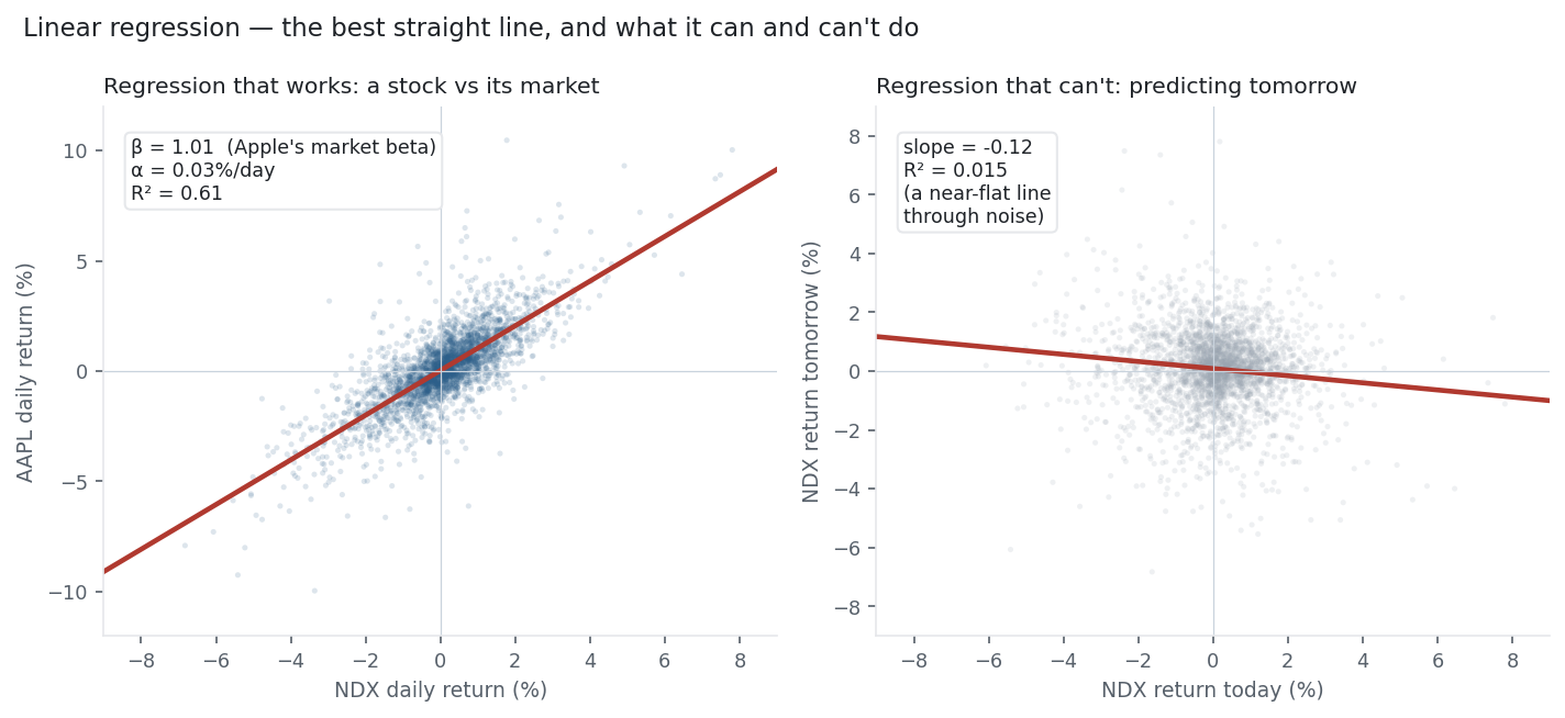
The left panel is the good news: regress Apple’s daily return on the Nasdaq’s and the fit is strong — β = 1.01 (Apple moves almost one-for-one with the index), α = 0.03%/day, and R² = 0.61, so 61% of Apple’s daily variance is explained by the market. That is a real, stable, tradeable relationship — the number every risk model uses. The right panel is the honest news: regress the Nasdaq’s return tomorrow on its return today and the line is nearly flat — slope −0.12, R² = 0.015. The same tool that captured Apple’s beta finds essentially nothing to predict about the market’s own next move. Linear regression measures the relationships that are there; it does not invent the ones that are not.
8. What does the Python code look like?
from sklearn.linear_model import LinearRegression
import numpy as np

# beta of Apple to the Nasdaq (X = market returns, y = stock returns)
model = LinearRegression().fit(X, y)
print(model.coef_[0], model.intercept_)     # -> 1.01 (beta), 0.03 (alpha, %/day)
print(model.score(X, y))                     # -> 0.61 (R^2)

# the same numbers, closed form, for one feature:
beta  = np.cov(x, y)[0, 1] / np.var(x, ddof=1)   # slope = cov / var
alpha = y.mean() - beta * x.mean()               # intercept
For inference (confidence intervals and p-values on the coefficients) use statsmodels.OLS, which prints the full regression table — but treat those p-values with suspicion on autocorrelated return data.
9. How would I explain it to a supervisor?
“Linear regression finds the straight line that minimises squared error, and for one feature its slope is just the covariance of x and y over the variance of x. Its coefficients are interpretable effect sizes, which is why it underpins CAPM and factor models. I use it as the baseline every more complex model must beat, and as a diagnostic: on the Nasdaq it recovers Apple’s beta cleanly (R² = 0.61), but it also shows — with an R² of 0.015 on next-day returns — that there is almost no linear signal to predict direction, exactly the efficient-market result. And I am careful with its inference on time series, because autocorrelation and volatility clustering violate its assumptions and inflate significance.”
Nasdaq-100 basket from the same multi_daily.csv used across the Equation Library (yfinance, adjusted closes). Both regressions (Apple-on-Nasdaq, and Nasdaq tomorrow-on-today) and the closed- form β = cov/var were computed and checked against the data.