Neural Networks
The multilayer perceptron — stacked nonlinear units that can approximate any function
This is where the library turns to deep learning. Every model so far had a fixed form — a line, a tree, a mixture of Gaussians. A neural network has almost no fixed form at all: it is a stack of simple units, each computing a weighted sum followed by a nonlinear squash, composed into layers deep enough to represent essentially any function. The humblest version is already familiar — a single neuron with a sigmoid is logistic regression. Stack many of those, feed the outputs of one layer into the next, and you get a multilayer perceptron (MLP): the foundation on which CNNs, RNNs, and transformers are all built. Its power is real and easy to demonstrate. Its limits, on the kind of data this site works with, are just as real — and worth being honest about.
1. What problem does it solve?
Supervised classification and regression, as a universal function approximator. Where a linear model assumes a straight relationship and a tree carves axis-aligned boxes, a neural network learns an arbitrary smooth mapping from inputs to output — and, crucially, learns its own intermediate features along the way (representation learning). It is the model class behind modern AI; the specialised architectures for images, text, and sequences are all neural networks with structure added.
2. What assumptions does it make?
Remarkably few — which is the point and the peril. It assumes only that the target is some function of the inputs that can be built by composing simple nonlinear units, and that you have enough data to pin down its many parameters. It makes no assumption of linearity, no distributional form, no independence. The flip side of assuming so little is needing so much: with weak priors, a network leans entirely on data, and given too little it will fit noise as happily as signal.
3. What data does it need?
Numeric, scaled inputs, and a lot of examples relative to its parameter count. Neural networks shine on high-dimensional, unstructured data — pixels, tokens, waveforms — where they learn representations no hand-engineering could match. On small-to-medium tabular data they are usually beaten by gradient boosting, which is the single most important practical fact about them for a quant: reach for a network when the data is large and unstructured, not by default.
4. How does it learn?
Start with the architecture. A neuron computes a weighted sum of its inputs plus a bias, then applies a nonlinear activation: a = g(w\cdot x + b). A layer is many neurons in parallel; a network stacks layers, each taking the previous layer’s outputs as its inputs. The forward pass just evaluates this composition. A tiny worked example — two inputs, two hidden ReLU units, one sigmoid output — makes it concrete. With x = (1,\ 2) and the hidden weights below:
z_1 = (0.5)(1) + (0.1)(2) = 0.7,\quad z_2 = (-0.2)(1) + (0.4)(2) = 0.6,
both survive the ReLU g(z)=\max(0,z), and an output neuron with weights (1,-1) and bias 0.2 gives z = (1)(0.7) + (-1)(0.6) + 0.2 = 0.3, so the prediction is \sigma(0.3) = 0.574.
The activation is what makes it work: without it, a stack of linear layers collapses algebraically into a single linear map — depth would buy nothing. With a nonlinearity between layers, the universal approximation theorem guarantees that even one hidden layer, given enough units, can approximate any continuous function. Training then sets the weights: define a loss (cross-entropy for classification, MSE for regression), compute its gradient with respect to every weight by backpropagation — the chain rule applied layer by layer, backwards — and take a step downhill with gradient descent (in practice SGD or Adam over mini-batches). The loss surface is non-convex, so this finds a local optimum, but with good initialisation and enough data it works remarkably well.
5. What are its strengths?
- Universal approximation. With enough capacity it can represent any continuous function — no functional form assumed.
- Representation learning. It discovers useful intermediate features automatically, instead of relying on hand-engineering.
- Scales with data and compute. Unlike most models, it keeps improving as you add data and parameters — the engine behind modern AI.
- State of the art on unstructured data. Images, audio, and language are its home turf.
- Composable and flexible. CNNs, RNNs, transformers are all neural networks with architectural structure added for a data type.
6. What are its weaknesses?
- Data- and compute-hungry. Many parameters need many examples and real hardware; starved of either, it overfits or underperforms.
- Overfits easily. Its flexibility fits noise as readily as signal — it needs regularisation (weight decay, dropout, early stopping) to generalise.
- Many hyperparameters. Architecture, learning rate, batch size, and regularisation all interact and demand tuning.
- A black box. The learned function is opaque; interpretability needs extra tooling.
- Usually loses on tabular data. For structured, modest-sized tables — most quant feature sets — gradient boosting typically wins with far less fuss.
7. How could it apply to markets?
The power is easy to show and the limits are easy to hit — both are in the figure. The left panel is the good news: on two interleaving “moons”, a straight logistic boundary manages 88% while an MLP bends around them for 96% — exactly the nonlinear separation the hidden layers buy you.
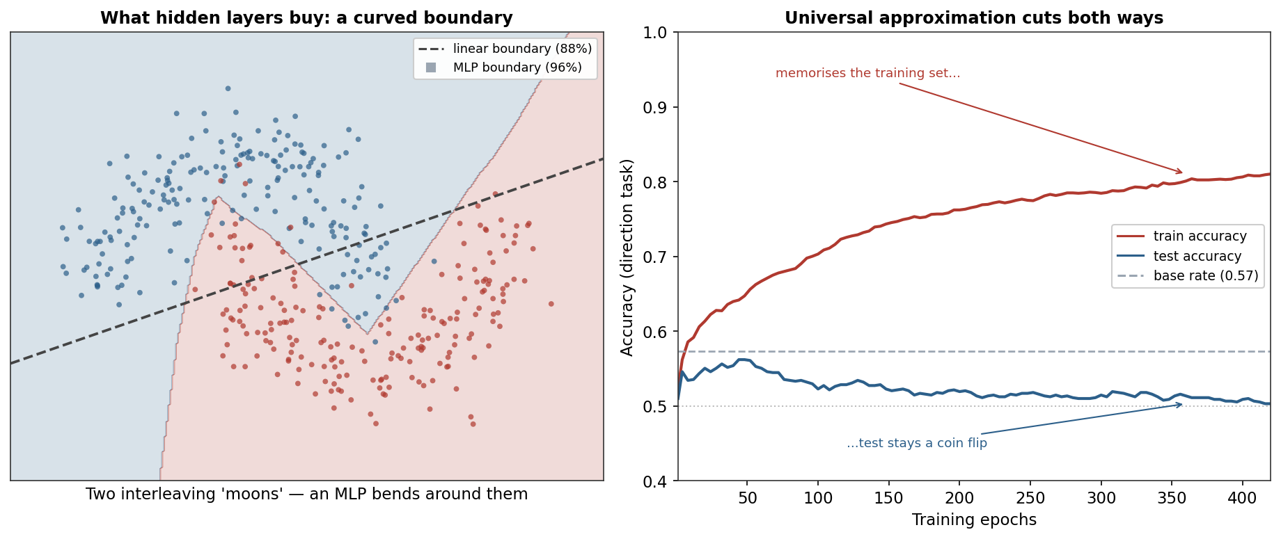
The right panel is the honest news. Put the same network on the tasks the tree models faced. On predicting a high-volatility day it reaches a test AUC of 0.56 — right alongside the random forest (0.57), gradient boosting (0.58), and even logistic regression (0.56). It finds the volatility-clustering signal, but it does not beat the simpler models; the universal approximator earns no premium where the structure is this mild. On predicting direction it becomes a cautionary tale. With over 1,200 parameters and only ~2,000 low-signal training rows, the network drives training accuracy above 80% while test accuracy drifts down to 0.50 — a coin flip, below the 0.57 base rate. It is memorising noise. (Notice the test curve peaks near epoch 40 and then decays: early stopping there would have salvaged its best, still-unremarkable, score.)
That is the lesson to carry into the rest of the deep-learning section. A neural network’s flexibility is a genuine superpower on the right data — but on small, noisy, tabular financial series it mostly supplies a faster route to overfitting. Its real edge is on unstructured market data — raw limit-order-book sequences, news text, tick-level waveforms — which is precisely what the specialised architectures ahead (CNNs, RNNs/LSTMs, transformers) are built to exploit. On a plain table of lagged returns, boosting remains the thing to beat.
8. What does the Python code look like?
from sklearn.neural_network import MLPClassifier
from sklearn.preprocessing import StandardScaler

X = StandardScaler().fit_transform(features)      # networks need scaled inputs

model = MLPClassifier(
    hidden_layer_sizes=(32, 16), activation="relu",   # two hidden layers
    alpha=1e-3,                                        # L2 weight decay (regularisation)
    early_stopping=True, n_iter_no_change=15,          # stop when validation stalls
    random_state=0).fit(X_train, y_train)

model.predict_proba(X_test)          # class probabilities from the output sigmoid/softmax
hidden_layer_sizes sets depth and width; alpha and early_stopping are the two regularisers that matter most on noisy data — turn them off on a series like this and you get the right-hand panel. For real deep learning (custom architectures, GPUs) you’d reach for PyTorch, but the moving parts — layers, activations, a loss, backprop, an optimiser — are identical.
9. How would I explain it to a supervisor?
“A neural network stacks layers of neurons, each computing a weighted sum passed through a nonlinear activation. The nonlinearity is essential — without it the layers collapse to a single linear map — and with it, one hidden layer is already a universal approximator. It’s trained by defining a loss, computing gradients with backpropagation, and stepping downhill with SGD or Adam; a single sigmoid neuron is just logistic regression. Its strength is representation learning on large, unstructured data, but it’s data-hungry and overfits easily. On the Nasdaq that’s exactly what I see: it matches the tree models on volatility at 0.56 AUC but doesn’t beat them, and on direction it pushes training accuracy past 80% while test collapses to a coin flip — its capacity buys memorisation, not signal. On tabular market data I’d still use boosting; the network’s edge is on unstructured data, which is what CNNs, RNNs, and transformers are for.”
Nasdaq-100 basket from the same multi_daily.csv as the Equation Library (yfinance, adjusted closes). scikit-learn MLPClassifier; the moons example uses make_moons. Volatility/direction tasks match the tree-model entries (70/30 time split, standardised features); the direction training curve is the network trained epoch-by-epoch (train ≈0.81, test ≈0.50, base rate 0.57). Forward-pass arithmetic and all figures were computed and checked.