Principal Component Analysis
Compressing many correlated features into a few uncorrelated directions of maximum variance
The second unsupervised model, and a different job from clustering. Where K-means groups the rows (which days are alike?), PCA reorganises the columns (which features move together?). It takes a set of correlated variables and finds a new set of axes — the principal components — that are uncorrelated with each other and ordered so the first captures as much of the data’s variance as possible, the second as much of what’s left, and so on. Because real data is usually redundant, a handful of these components reproduces almost all of it, so you can throw the rest away. It is the workhorse of dimensionality reduction — and on a basket of stocks it produces one of the most satisfying results in quantitative finance: the first component is the market.
1. What problem does it solve?
Dimensionality reduction — collapsing many correlated features into a few informative ones — and, along the way, decorrelation (the new features are orthogonal), visualisation (project high- dimensional data to 2-D), compression, and denoising (low-variance components are often noise). It is unsupervised: there is no target, only the structure of the features themselves. You reach for it when features are numerous and correlated, and you want a smaller, cleaner set before modelling — or when you want to understand what common factors drive a dataset.
2. What assumptions does it make?
Three, and they define its limits. First, that variance equals information — the directions worth keeping are the high-variance ones, which is true for signal but can fail if the interesting structure is low-variance. Second, that the structure is linear: components are linear combinations of the original features, so PCA can’t capture curved manifolds (kernel PCA or autoencoders are the nonlinear answers). Third, that features are on comparable scales — because it chases variance, an unscaled large-variance feature dominates every component, so you almost always standardise (z-score) first, which makes PCA operate on the correlation matrix rather than the covariance matrix.
3. What data does it need?
Numeric, standardised features that are correlated — if features are already independent, there is nothing to compress and PCA does nothing useful. It shines on redundant, collinear data (factor models, sensor arrays, image pixels, term structures). It is sensitive to outliers (they inflate variance and tilt the components) and, being a variance method, it is happiest when the features are roughly elliptically distributed.
4. How does it learn?
PCA has no iterative training — it’s a single linear-algebra step. Standardise the data, form the covariance/correlation matrix \Sigma, and take its eigen-decomposition:
\Sigma\, v_i = \lambda_i\, v_i .
Each eigenvector v_i is a principal component — a direction in feature space — and its eigenvalue \lambda_i is the variance of the data along that direction. Sort the eigenvectors by eigenvalue, largest first, and you have the components ordered by importance; the fraction \lambda_i / \sum_j \lambda_j is the variance explained by component i. (In practice libraries use the SVD of the data matrix, which is numerically better but gives the same result.) Project the data onto the top few eigenvectors and you’ve reduced its dimension while keeping the most variance possible.
A tiny worked case shows it exactly. For two standardised, correlated features with covariance \Sigma = \left(\begin{smallmatrix} 2 & 1 \\ 1 & 2 \end{smallmatrix}\right), solving \det(\Sigma - \lambda I) = 0 gives \lambda = 3 and \lambda = 1. The first component points along (0.707,\ 0.707) — the 45° line the two correlated features share — and explains 3/(3+1) = 75\% of the variance; the second, orthogonal at (0.707,\ -0.707), mops up the remaining 25%. Two features became one meaningful axis plus a remainder.
5. What are its strengths?
- Removes multicollinearity. The components are orthogonal by construction — ideal as inputs to models that hate correlated features.
- Compresses with little loss. A few components usually reproduce the bulk of the variance, shrinking the problem.
- Denoises. Dropping the smallest components often discards mostly noise, stabilising downstream models.
- Fast and deterministic. One eigen/SVD computation — no tuning, no random restarts, a unique answer.
- Interpretable factors, sometimes. When the components line up with real structure (as below), they mean something.
6. What are its weaknesses?
- Components can be hard to read. Each is a blend of every original feature; unless the loadings are clean, “PC4” resists interpretation.
- Unsupervised — max variance ≠ max signal. The highest-variance direction need not be the one that predicts your target; PCA optimises the wrong objective for that (partial least squares doesn’t).
- Linear only. It captures linear correlation, missing curved structure (use kernel PCA / autoencoders).
- Scale- and outlier-sensitive. Skip standardisation and one feature dominates; a few outliers can hijack a component.
- Discards low-variance directions blindly. Occasionally the small-variance component is the informative one, and PCA throws it out.
7. How could it apply to markets?
PCA is everywhere in quant finance: extracting risk factors from a universe of returns, decorrelating features before a model, and the textbook yield-curve decomposition into level, slope, and curvature. To show what it finds, I ran it on the daily returns of five names — the Nasdaq-100 index and AAPL, MSFT, NVDA, PEP — standardised, over ~2,900 days (their average pairwise correlation is 0.54, so there is plenty of shared structure to compress).
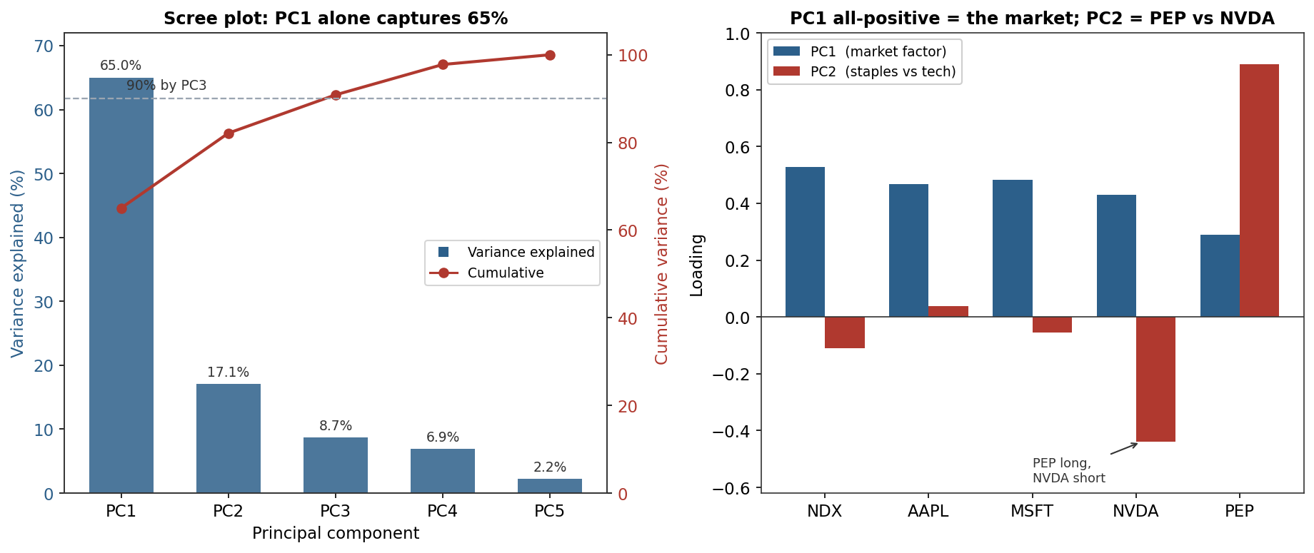
The result is the classic one. PC1 explains 65% of the variance and loads positively on every asset (0.29 to 0.53) — it is the market factor, the common up-and-down that moves everything together, and each asset’s loading is essentially its sensitivity to it, the same idea as its market beta. PC2 (17%) is a clean contrast: strongly positive on PEP (+0.89), negative on NVDA (−0.44), roughly flat elsewhere — defensive consumer-staples behaviour versus high-beta semiconductors, the second-biggest driver of how these names diverge. Three components account for 91% of the variance, so five correlated series are, for practical purposes, three underlying factors plus noise. This is PCA earning its place: it took a redundant basket and handed back an interpretable, low-dimensional description of what actually moves it — genuine, unlike the direction-prediction dead-ends elsewhere on this site, because variance (unlike tomorrow’s sign) is real and structured.
8. What does the Python code look like?
from sklearn.decomposition import PCA
from sklearn.preprocessing import StandardScaler

X = StandardScaler().fit_transform(returns)        # standardise FIRST (PCA chases variance)
pca = PCA().fit(X)

pca.explained_variance_ratio_     # variance each component captures -> the scree plot
pca.components_                    # the eigenvectors: loadings of each PC on the features
scores = pca.transform(X)         # data projected onto the components (the reduced features)

PCA(n_components=0.90).fit(X)      # or: keep just enough components for 90% of the variance
explained_variance_ratio_ is the number you actually look at (how many components to keep); components_ holds the loadings you interpret; transform gives the reduced representation to feed downstream. Passing a float like 0.90 lets scikit-learn pick the component count for you.
9. How would I explain it to a supervisor?
“PCA is unsupervised dimensionality reduction. You standardise the features, take the eigen- decomposition of their correlation matrix, and the eigenvectors are new orthogonal axes — the principal components — ordered by eigenvalue, which is the variance along each. Keep the top few and you’ve compressed the data with minimal loss, and decorrelated it as a bonus. The caveat is that it’s unsupervised, so the highest-variance direction isn’t necessarily the most predictive, and it’s linear. The nice demonstration is on stock returns: on a five-asset Nasdaq basket, PC1 explains 65% and loads positively on everything — that’s the market factor, essentially the assets’ betas — and PC2 sets PEP against NVDA, staples versus tech. Three components cover 91%. It’s the honest kind of result this data gives up: variance has real structure, even though direction doesn’t.”
Five daily return series (NDX, AAPL, MSFT, NVDA, PEP) from the same multi_daily.csv as the Equation Library (yfinance, adjusted closes), ~2,900 observations, standardised. PCA via scikit-learn; explained-variance ratios and component loadings computed directly and checked, with the 2×2 eigen example worked by hand above. Component signs are arbitrary (fixed so PC1 is positive).