Probability Calibration & Conformal Prediction
Honesty, not skill — making a model’s probabilities mean what they say, and its intervals cover what they promise
Every model in this library outputs a number that looks like a probability or a forecast — but a system that sizes positions by confidence needs those numbers to be true, not just plausible. This entry is about that truth, and it splits cleanly in two. Calibration asks whether a model’s stated probabilities match reality: when it says 70%, does the event happen 70% of the time? Conformal prediction asks the same of intervals: does a “90% interval” actually contain the outcome 90% of the time — provably, without assuming a distribution? Both matter enormously here precisely because this site’s central finding is that next-day direction is unpredictable (AUC ≈ 0.50 everywhere). A no-skill model is not the problem; a dishonest one is. A model that shrugs and says “50/50” is safe; a model that confidently says “84% up” when it is really a coin toss is how an automated system blows up. Calibration and conformal prediction are the tools that enforce honesty on top of whatever skill — or lack of it — a model actually has. They are the proposal’s trustworthiness layer.
1. What problem does it solve?
Making uncertainty trustworthy. A raw model score is often not a real probability: gradient-boosted trees and neural nets are frequently over-confident (pushing scores toward 0 and 1), over-fit models especially so. If a downstream system multiplies “probability of up” by a position size, or treats a forecast interval as a risk limit, then miscalibrated confidence translates directly into mis-sized risk. Calibration fixes the probabilities; conformal prediction attaches a guarantee to the intervals. Together they let every probabilistic output in the architecture be taken at face value — or, where it cannot be, flagged honestly as uncertain.
2. Calibration — making probabilities mean what they say
A classifier is calibrated if, among all the times it says p, the event occurs a fraction p of the time. Miscalibration is measured, not eyeballed. The reliability diagram plots predicted probability against empirical frequency — perfect calibration is the diagonal. The Expected Calibration Error summarises the gap,
\text{ECE} \;=\; \sum_{b=1}^{B} \frac{n_b}{n}\,\big|\,\text{acc}_b - \text{conf}_b\,\big|,
the bin-weighted distance between confidence and accuracy, and the Brier score \frac{1}{n}\sum_i (p_i - y_i)^2 scores the full probabilistic prediction (it decomposes, by Murphy’s identity, into reliability − resolution + uncertainty — calibration improves the reliability term). Two standard recalibrators fix a miscalibrated model using a held-out calibration set: Platt scaling fits a logistic sigmoid to the scores (one slope, one intercept — robust, low-variance), and isotonic regression fits an arbitrary monotone step function (flexible, but data-hungry and prone to over-fit small sets). Both are monotone, which is the key to the next point.
3. An over-confident no-skill model, made honest
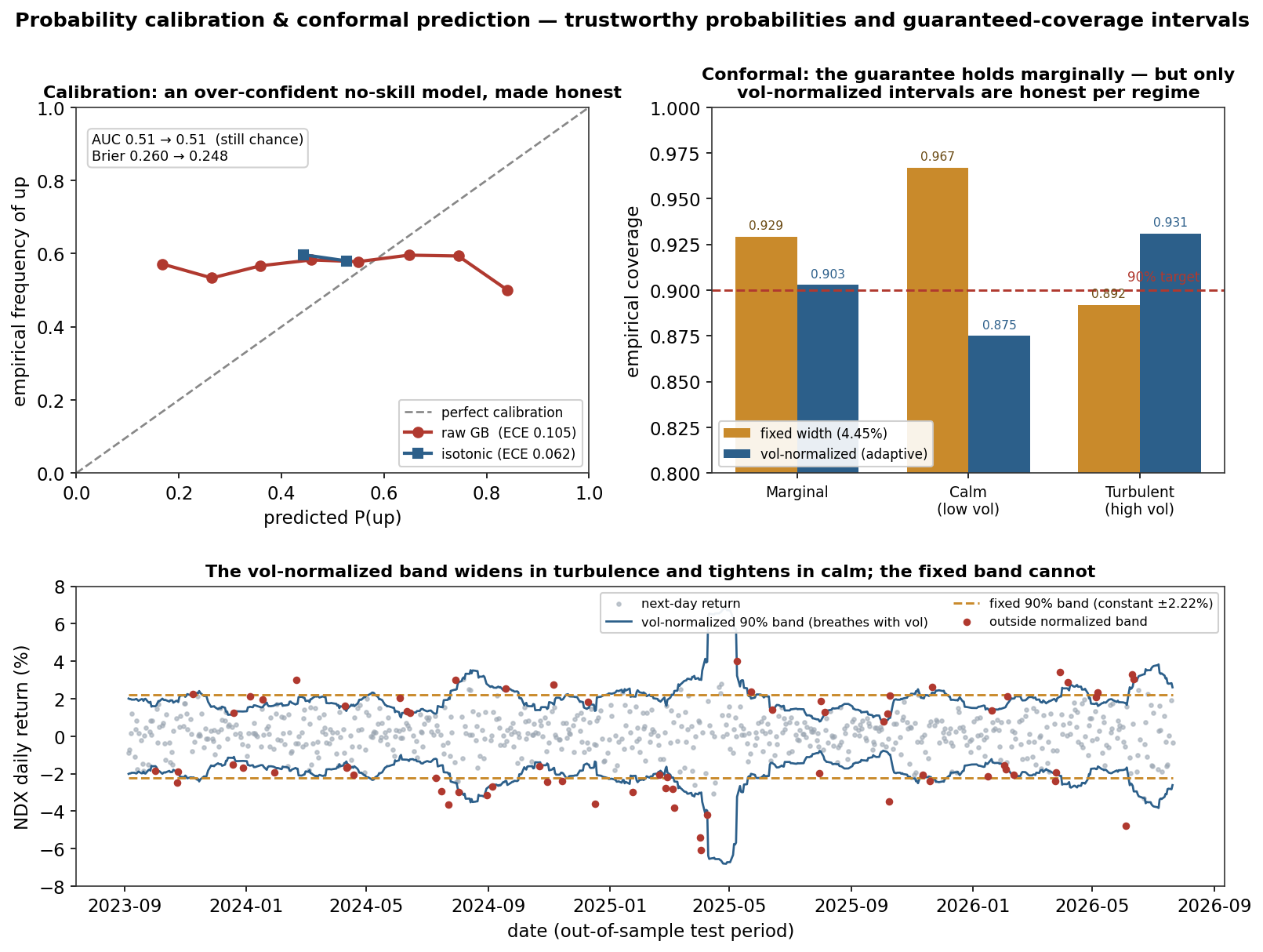
The left panel trains a gradient-boosted classifier to predict next-day Nasdaq direction — a task this site has shown again and again has essentially no signal. The model duly earns AUC 0.512: chance. Yet its raw probabilities range from 0.16 to 0.94 — wildly over-confident for a coin toss — and its reliability curve sags well below the diagonal, an ECE of 0.105. Isotonic recalibration on a chronological hold-out pulls the curve onto the diagonal, roughly halving ECE to 0.062 and improving the Brier score from 0.260 to 0.248. Crucially, AUC is unchanged at 0.51: because recalibration is monotone, it cannot reorder the predictions, so it adds no discriminative skill and removes none. That is the whole subtle lesson — calibration is not skill. The two are orthogonal virtues: a model can be perfectly calibrated and useless (always predict the base rate), or skilful and badly miscalibrated. You must measure both, and here calibration makes an honest, humble model out of an over-confident one without pretending it can predict the market. One honest counter-result sharpens the rule: the same recalibration applied to an already-calibrated random forest (raw ECE 0.020) made it worse (0.059) — isotonic regression over-fit the small calibration set. Recalibration is not free; it needs a genuinely miscalibrated model and enough calibration data.
4. Conformal prediction — a coverage guarantee without distributional assumptions
Calibration disciplines probabilities; conformal prediction disciplines intervals, and it does so with a remarkable guarantee: under exchangeability alone — no Gaussianity, no model correctness — a split-conformal interval covers the truth with probability at least 1-\alpha in finite samples. The recipe is disarmingly simple. Hold out a calibration set, compute a nonconformity score for each point (for a point forecast \hat\mu, just the residual s_i = |y_i - \hat\mu_i|), take the empirical quantile at level \lceil (n+1)(1-\alpha)\rceil / n, and use it as the interval half-width. The right panels test this on next-day Nasdaq returns at a 90% target: the marginal coverage lands at 0.929 (fixed) — the guarantee holds. But marginal coverage is not conditional coverage, and this is where markets bite. A constant-width interval over-covers calm days (96.7% — needlessly wide) and under-covers turbulent ones (89.2% — too narrow exactly when a tail is dangerous), because returns are heteroskedastic: volatility clusters, so one width cannot serve both regimes. Normalizing the nonconformity score by a predicted volatility, s_i = |y_i - \hat\mu_i| / \hat\sigma_i, makes the interval breathe — half-width \hat q\,\hat\sigma_t, narrow in calm (±1.5%) and wide in turbulence (beyond ±7%, bottom panel). It holds 90.3% marginal coverage and brings both regimes near target (0.875 / 0.931), with the exceptions now scattered through time rather than piled up in the crises. The guarantee was always distribution-free; normalization makes it regime-honest.
5. What are its strengths?
- Honesty is separable from skill. Calibration makes a model’s confidence trustworthy whatever its (possibly nonexistent) predictive power — exactly what a risk-sizing system needs.
- Conformal’s guarantee is distribution-free and finite-sample. No Gaussian assumption, no correct-model assumption — just exchangeability — which is rare and valuable.
- Model-agnostic wrappers. Both sit on top of any classifier or regressor, so every model in the library can be made trustworthy without being rebuilt.
- Cheap and interpretable. A reliability diagram, an ECE, a coverage number — quantities a risk committee can read and audit directly.
- Normalization ties it to regime. Vol-scaled conformal reuses this site’s volatility and regime machinery to make intervals conditionally honest.
6. What are its weaknesses?
- Recalibration can hurt. On an already-calibrated model or a small calibration set it adds variance — the random-forest counter-result — so it must be checked, not assumed.
- Markets are not exchangeable. Conformal’s guarantee assumes exchangeability; non-stationary, vol-clustered returns violate it, so coverage is approximate (0.929, not exactly 0.90) and needs adaptive or normalized variants.
- Marginal ≠ conditional. The headline guarantee is average coverage; without normalization the interval can be systematically wrong in the regime that matters, as shown.
- Calibration is only to the calibration distribution. A regime shift after calibration breaks it — the same distribution-shift Achilles’ heel as everything in this library.
- Isotonic over-fits; Platt can under-fit. The recalibrator is itself a model with bias–variance trade-offs and needs enough held-out data.
7. How could it apply to markets?
This is the proposal’s trustworthiness layer, and it serves two agents directly. The News & Narrative Agent emits probabilities — event likelihoods, sentiment confidences, direction odds — and if those are miscalibrated, every downstream decision that multiplies by them is mis-scaled; calibration is what lets the rest of the system take them at face value. The Risk Agent lives on intervals: a VaR or expected-shortfall limit is a coverage statement, and conformal prediction gives it a distribution-free backing rather than a fragile Gaussian assumption. The demonstration’s lesson is the design’s: a fixed interval is conditionally dishonest, so the Risk Agent’s intervals must be vol- and regime-normalized — which is exactly why this layer sits downstream of the regime, change-point and volatility models rather than beside them. And the sharpest point is the one that runs through the whole site: because direction is unpredictable, the most valuable thing a model can do is know that it doesn’t know — a calibrated 0.50 and an interval that widens honestly in turbulence are worth more than any confident forecast the market will not honour. As always, the machinery was checked against its guarantee — a known 90% target, coverage measured — before being trusted.
8. What does the Python code look like?
import numpy as np
from sklearn.isotonic import IsotonicRegression

# --- Calibration: fit a monotone map on a held-out calibration set, apply to test ---
iso   = IsotonicRegression(out_of_bounds="clip").fit(p_calib, y_calib)   # scores -> honest probs
p_hat = iso.predict(p_test)                                              # AUC unchanged (monotone)

def ece(p, y, B=15):                          # expected calibration error
    b = np.linspace(0, 1, B + 1); e = 0.0
    for j in range(B):
        m = (p >= b[j]) & (p < b[j+1] if j < B-1 else p <= b[j+1])
        if m.sum(): e += m.mean() * abs(y[m].mean() - p[m].mean())
    return e

# --- Split conformal: distribution-free 90% interval, vol-normalized so it is regime-honest ---
alpha = 0.10
scores = np.abs(y_calib - mu_calib) / sig_calib          # normalized nonconformity (sig = predicted vol)
level  = np.ceil((len(scores)+1)*(1-alpha)) / len(scores)
q      = np.quantile(scores, min(level, 1.0), method="higher")
lo, hi = mu_test - q*sig_test,  mu_test + q*sig_test      # half-width q*sigma_t -> breathes with vol
coverage = np.mean((y_test >= lo) & (y_test <= hi))       # verify against the 0.90 target
The two ideas share a shape: hold out data the model never trained on, and use it to measure and correct the model’s honesty — probabilities in the first case, interval widths in the second.
9. How would I explain it to a supervisor?
“Two ideas about trustworthy uncertainty. Calibration: a model’s probabilities should match reality — when it says 70%, it should be right 70% of the time. I trained a gradient-boosted model on next-day Nasdaq direction; it has no skill, AUC 0.51, but its raw probabilities ranged from 0.16 to 0.94 — wildly over-confident — with a calibration error of 0.105. Isotonic recalibration halved that to 0.062 and improved the Brier score, and because it’s monotone the AUC didn’t move at all — which is the key point, calibration is honesty, not skill; they’re orthogonal and you measure both. There’s an honest caveat: recalibrating an already-calibrated random forest made it worse, so it’s not free. Second, conformal prediction: under exchangeability alone — no distributional assumption — a split-conformal interval has a guaranteed coverage. I built a 90% interval for next-day returns and it covered 93% marginally, so the guarantee holds. But a constant-width interval over-covered calm days at 97% and under-covered turbulent days at 89%, because volatility clusters; normalizing the score by predicted volatility makes the band breathe — narrow in calm, wide in a crisis — and restores about 90% in both regimes. For my proposal this is the trustworthiness layer: it makes the News Agent’s probabilities safe to act on and gives the Risk Agent distribution-free, regime-adaptive intervals instead of a fragile Gaussian VaR. The theme of the whole site is here too — because direction is unpredictable, the most valuable thing a model can do is know that it doesn’t know.”
Calibration: gradient-boosted classifier (400 trees) on next-day NDX direction, 8 past-only features, chronological train/calibration/test split (1586 / 577 / 721). Raw AUC 0.512, ECE 0.105, Brier 0.2605; after isotonic AUC 0.506, ECE 0.062, Brier 0.2480 (Platt: ECE 0.059, Brier 0.2470); random-forest counter-result raw ECE 0.020 → 0.059. ECE with 15 equal-width bins. Conformal: split conformal on next-day NDX returns, \hat\mu=0, \hat\sigma_t = 20-day trailing volatility (no leakage), \alpha=0.10, finite-sample quantile level \lceil(n{+}1)(1{-}\alpha)\rceil/n. Marginal coverage fixed 0.929 / normalized 0.903; conditional (median-vol split) fixed 0.967 (calm) / 0.892 (turbulent), normalized 0.875 / 0.931; mean width fixed 4.45% (constant) vs normalized 4.21% (adaptive, ≈3.1% calm → 5.3% turbulent). Every number was checked.