Supervised Liquidity-Stress Modelling

Forecasting stress ahead from labelled outcomes — and finding that a single transparent volatility feature beats the classifier: the supervised counterpart to the liquidity tripwire

The supervised half of the liquidity specialist: a gradient-boosted classifier that forecasts whether the coming week will be a stress week, evaluated with purged walk-forward. It beats chance handsomely (average precision 0.46 against a 15% base rate, ROC-AUC 0.80) and is well calibrated (Brier 0.106) — but ranking days by a single transparent feature, today’s 20-day realised volatility, beats it (AP 0.49, ROC-AUC 0.83). Forward-stress predictability is volatility persistence; the supervised label buys a calibrated probability, not incremental timing.

The liquidity-stress anomaly detector answers one question — is today abnormal? — without labels, by learning the shape of normal conditions. This entry is its supervised twin, and it answers the forward-looking question the unsupervised detector cannot: how likely is the coming week to be stressed, and how severe? Give the market a label — a stress week — and you can train a classifier to forecast it and, more usefully, to emit a calibrated probability. The entry builds that classifier honestly, and its most important result is a null: the supervised model, on seven features, does not beat ranking days by a single transparent feature — today’s realised volatility. It is the site’s recurring lesson in the liquidity domain — adaptive machinery pays only in proportion to the structure it can exploit beyond a transparent baseline, and here that structure is just volatility persistence.

1. What problem does this model solve?

Forecasting imminent liquidity/volatility stress from labelled outcomes, with a calibrated probability. The anomaly detector nowcasts a condition; a supervised model can forecast one, because a label lets you point today’s features at tomorrow’s outcome. That buys two things the unsupervised score cannot give the risk layer: a probability on a known scale — “there is a 40% chance the next week is a stress week” — and, if the label encodes severity, an expected magnitude. The honest question this entry is built to answer is not “can it forecast stress?” (volatility clusters, so of course something can) but “does the labelled, multi-feature machine beat the obvious one-line baseline of using current volatility?” — the only version of the question that decides whether the model earns its place.

2. What assumptions does it make?

A usable label exists: here, a stress week is one whose forward five-day realised volatility lands in the top decile of the training window — rare, so this is an imbalanced problem where accuracy is meaningless and precision–recall and calibration are the right lenses. Point-in-time features: every input is known at the close of day t; the label looks only at t{+}1\ldots t{+}5. No overlapping-label leakage: because the five-day forward window makes adjacent labels overlap, the train/test split must be purged and embargoed or the model simply reads the answer — the classic data-leakage trap in financial ML. And enough stationarity that a threshold learned on the past is meaningful in the future — an assumption the data itself strains, as the weakness section shows.

3. What data does it need?

The same daily Nasdaq-100 OHLCV as the unsupervised detector, and the same stress-feature family, so the two are a fair pair: intraday range (H-L)/C, absolute return |r|, overnight gap, a 20-day volume z-score, and an Amihud illiquidity measure |r|/(V/\bar V_{20}) — plus short realised-volatility history (trailing 5- and 20-day). The label is built from forward five-day realised volatility. Genuine liquidity again lives in spreads, depth and order flow the daily bars only proxy; the point here is the method and its honest evaluation, which transfer directly to a richer feed.

4. How does it learn?

A gradient-boosted tree classifier (histogram boosting) is fit on the labelled feature panel, and evaluated by purged, embargoed walk-forward — an expanding window with a five-day gap between train and test, so no training row shares its forward window with a test row. The stress threshold is taken from the training fold only and applied out of sample, so the label is never defined with future information. The model returns a probability per day; the decision layer flags, say, the top decile of predicted probabilities. Against it runs the baseline it must beat: rank each day by its current 20-day realised volatility — no training, no labels, one feature.

Panel A: out-of-sample calibration — predicted stress probabilities track observed frequencies down the diagonal, Brier 0.106. Panel B: precision–recall for forecasting next-week stress — the supervised classifier on all seven features (blue, average precision 0.46) is matched or beaten across the curve by ranking on today’s 20-day realised volatility alone (amber, 0.49), both far above the 15% base rate. Panel C: the model’s predicted stress probability over 2017–2026, with realized stress weeks (red) clustering under the probability spikes — it fires around real stress, it just does not beat the volatility signal it is mostly rediscovering.

5. What are its strengths?

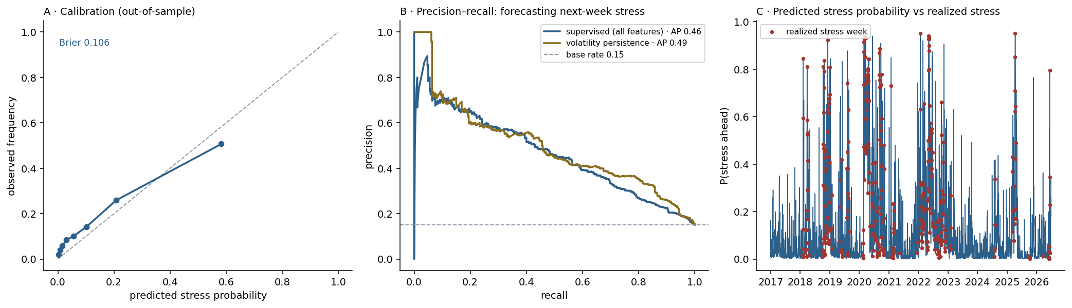
• It forecasts, and it is calibrated. Out of sample the model reaches average precision 0.46 against a 15.1% base rate — a 3.1× lift — with ROC-AUC 0.80, and its probabilities are trustworthy: Brier 0.106 and a reliability curve that hugs the diagonal. A calibrated P(\text{stress ahead}) is exactly what the risk layer can act on, and it is something the unsupervised anomaly score cannot supply.
• Economically real. Days in the top decile of predicted probability are followed by 35.6% realised volatility versus 17.4% after the rest — a 2.0× separation — so the score genuinely leads danger.
• Labels enable severity and thresholds. Unlike an anomaly score with no natural units, a supervised target can encode how bad and be tuned to an explicit precision–recall operating point (here, flagging the top decile gives precision 0.56, recall 0.37).
• Honest by construction. Purged walk-forward, PR-AUC against the base rate, and calibration make the evaluation leakage-resistant and imbalance-aware — the discipline is part of the result.

6. What are its weaknesses?

• It does not beat one transparent feature — the headline. Ranking days by today’s 20-day realised volatility alone scores AP 0.49 and ROC-AUC 0.83, above the seven-feature classifier (0.46, 0.80); a microstructure-only model with no volatility history manages 0.44. The predictable part of forward stress is volatility persistence, and the ML machinery mostly rediscovers it — at best matching, here slightly trailing, the honest baseline. This is the vol-forecasting-horizon lesson in classifier form.
• Overlapping labels are a leakage trap. The forward window makes adjacent labels correlated; without the embargo the same scores balloon spuriously — a reminder that in this setting the validation design matters more than the model.
• Non-stationarity moves the target. Trained on calmer years, the model meets a market where stress weeks are 15% of out-of-sample days, not the 10% the threshold was set for — a drifting base rate that mis-scales any fixed cut-off.
• Imbalanced and directionless. Accuracy is meaningless at a 15% base rate, so it must be read through precision–recall and calibration; and like its unsupervised twin it forecasts stress, not direction or cause.

7. How could it apply to markets?

In the proposal this is the supervised, forecasting half of the liquidity specialist, paired with the unsupervised nowcasting detector: the anomaly score says the market is abnormal now, the classifier says the coming week is likely to be stressed, with this calibrated probability. Both feed the risk-on/off verdict and the deterministic risk layer. But the null disciplines the design rather than killing the model. Because a transparent volatility signal is as good a forecaster, the system should treat current volatility as the benchmark the classifier must beat — the same fair-baseline principle the proposal’s research question is built on — and value the supervised model for what it does add: a calibrated probability on a known scale, multi-feature robustness when volatility alone is ambiguous, and a natural home for severity and richer order-book features a one-feature rule cannot use. It is another instance of the site’s thesis: market-state information is a calibration and risk-control signal, not a source of timing alpha beyond what a simple, transparent measure already provides.

8. What does the Python code look like?

import numpy as np, pandas as pd
from sklearn.ensemble import HistGradientBoostingClassifier
from sklearn.model_selection import TimeSeriesSplit
from sklearn.metrics import average_precision_score, roc_auc_score, brier_score_loss

# label: is the coming week a stress week? forward 5-day realised vol, top decile
fwd = r.rolling(5).std().shift(-5) * np.sqrt(252)          # std of r[t+1 .. t+5]

proba = np.full(len(X), np.nan)
for tr, te in TimeSeriesSplit(n_splits=5, gap=5).split(X):  # purged + embargoed
    thr = np.quantile(fwd[tr], 0.90)                        # threshold from TRAIN only
    y_tr = (fwd[tr] >= thr).astype(int)
    model = HistGradientBoostingClassifier(max_depth=3, learning_rate=0.05,
                                           max_iter=300, l2_regularization=1.0)
    model.fit(X[tr], y_tr)
    proba[te] = model.predict_proba(X[te])[:, 1]

y = (fwd >= threshold_per_fold).astype(int)
ap_model   = average_precision_score(y, proba)             # 0.46
ap_persist = average_precision_score(y, rv20)              # 0.49  <- one feature wins
brier      = brier_score_loss(y, proba)                    # 0.106, well calibrated

The label and the purged split are the substance; the classifier is almost incidental, which is the result.

9. How would I explain it to a supervisor?

“This is the supervised counterpart to my unsupervised liquidity detector. I labelled a stress week as one whose next-five-day realised volatility is in the top decile, and trained a gradient-boosted classifier to forecast it from daily stress features, evaluated with purged, embargoed walk-forward so the overlapping forward windows can’t leak. It works: out of sample it reaches average precision 0.46 against a 15% base rate — a 3× lift — with ROC-AUC 0.80, it’s well calibrated at Brier 0.106, and the week after a high-probability day realises 36% volatility versus 17% otherwise. But the honest result is a null: if I just rank days by today’s 20-day realised volatility — one feature, no model — I get 0.49 and 0.83, better than the classifier. Forward stress is predictable, but the predictable part is volatility persistence, and the machine mostly rediscovers it. So I don’t present this as alpha; I present it as a calibrated probability the risk layer can use, benchmarked honestly against the vol signal it has to beat — which is exactly the fair-baseline standard my whole proposal is built on.”

NDX daily 2015–2026 (equations/ndx_daily.csv). Features (point-in-time at close of t): range (H-L)/C, |r|, overnight gap, 20-day volume z-score, Amihud |r|/(V/\bar V_{20}), trailing 5- and 20-day realised volatility. Label: forward five-day realised volatility \ge the training-fold 90th percentile. Evaluation: TimeSeriesSplit(n_splits=5, gap=5) purged/embargoed walk-forward, 2,385 out-of-sample days, base rate 15.1%. Histogram gradient-boosted classifier (max_depth 3, lr 0.05, 300 iters, L2 1.0): average precision 0.464, ROC-AUC 0.799, Brier 0.106; top-decile flag precision 0.556, recall 0.369; forward vol 35.6% (high-probability) vs 17.4% (rest). Microstructure-only model AP 0.435. Volatility-persistence baseline (rank by trailing 20-day realised volatility): AP 0.493, ROC-AUC 0.827 — above the classifier. Every number was checked.