Support Vector Machines
The maximum-margin classifier — and the kernel trick for nonlinear boundaries
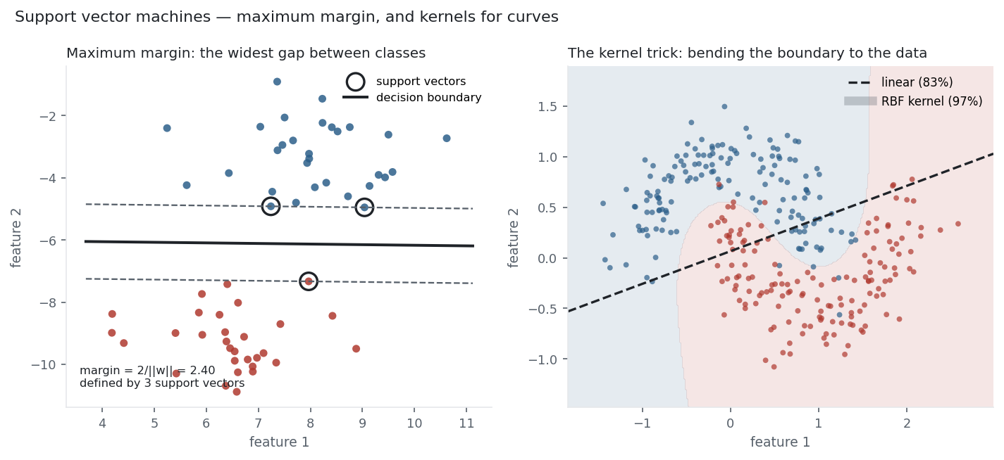
A support vector machine draws the boundary between two classes not just somewhere between them, but in the single best place: the position with the widest margin — the largest gap to the nearest points of either class. The intuition is that a boundary sitting in the middle of a wide no-man’s-land generalises better than one squeezed against the data. Only the points on the edge of that gap — the support vectors — actually matter; everything else could move and the boundary wouldn’t budge. And through the kernel trick, the same idea draws curved boundaries without ever computing the curve. It is one of the most elegant models in machine learning, and a useful contrast to the logistic regression and tree families.
1. What problem does it solve?
Primarily binary classification (multi-class by combining one-vs-rest classifiers), and regression too (as SVR). It excels on medium-sized, high-dimensional problems — text, genomics, and any setting where the number of features rivals or exceeds the number of samples — where its margin-maximising, support-vector-based fit resists overfitting.
2. What assumptions does it make?
That a good boundary exists — either directly, or after a kernel lifts the data into a higher-dimensional space where it becomes separable — and that the maximum-margin boundary is the one that generalises. It makes no probabilistic model of the data (it outputs a decision, not a calibrated probability, unless you add Platt scaling). Crucially it assumes features are on comparable scales, because the margin is measured by Euclidean distance — unscaled features silently dominate.
3. What data does it need?
Numeric, scaled features and a modest number of rows. Kernel SVMs cost roughly O(n^2)–O(n^3) to train, so they are happiest up to tens of thousands of samples, not millions — which is why trees and boosting have displaced them on big tabular data. Where they still shine is high-dimensional data, comfortably handling more features than samples.
4. How does it learn?
It maximises the margin, which is equivalent to minimising \tfrac{1}{2}\|w\|^2 subject to every point being on the correct side by at least a unit distance, y_i(w\cdot x_i + b) \ge 1. Real data isn’t perfectly separable, so the soft-margin version allows violations, penalised by a parameter C: large C insists on few violations (a hard margin that can overfit), small C tolerates more (a wider, more regularised margin). Written as a loss, the SVM minimises the hinge loss plus an L2 penalty:
\min_w\ \underbrace{\sum_i \max\!\big(0,\ 1 - y_i\,f(x_i)\big)}_{\text{hinge loss}} \;+\; \lambda\,\|w\|^2,
where f(x) = w\cdot x + b. The hinge loss charges nothing for points classified correctly and beyond the margin, and grows linearly once they cross it — so maximising the margin is just L2 regularisation in disguise. The optimisation (a quadratic program) turns out to depend on the data only through inner products x_i\cdot x_j, which is the opening for the kernel trick: replace that inner product with a kernel K(x_i, x_j) — polynomial, or the Gaussian RBF — and you get the max-margin boundary in a high-dimensional feature space without ever computing the coordinates there. That is how the right panel of the figure bends a straight boundary into a curve.
5. What are its strengths?
- Strong in high dimensions. Works even when features outnumber samples, where many models fail.
- Defined by a few support vectors. The model is compact and depends only on the boundary points — robust to points far from the margin.
- Nonlinear via kernels. The RBF kernel draws arbitrarily curved boundaries with one extra parameter.
- Max-margin generalises. The widest-gap principle gives good out-of-sample behaviour with the right C.
- Well-founded. Convex optimisation (a global optimum) and clean theory (VC dimension, margins).
6. What are its weaknesses?
- Scales badly. O(n^2)–O(n^3) training makes kernel SVMs impractical on large datasets — the main reason boosting has overtaken them.
- Needs scaling and tuning. Features must be standardised, and C and the kernel’s \gamma strongly affect results.
- No native probabilities. It returns a margin/decision; calibrated probabilities require Platt scaling or isotonic regression.
- Opaque with kernels. A linear SVM’s weights are readable; an RBF SVM is a black box.
- Sensitive to noise near the boundary. Because support vectors are the boundary points, mislabelled points there distort it.
7. How could it apply to markets?
SVMs suit smaller, high-dimensional market problems — classifying regimes or events from many engineered features, where the sample count is modest but the feature count is large — and were popular for exactly this before boosting scaled better. On the standard tasks they behave like the other models here.
Put an SVM to the same volatility and direction tests as the tree models (features standardised first, as SVMs require). On predicting a high-volatility day it reaches a test AUC of 0.57 — linear and RBF kernels both — matching the random forest and boosting: the volatility-clustering signal is real and every capable model finds it. On predicting direction, the RBF SVM manages AUC 0.51, no better than a coin flip. The margin machinery and the kernel trick don’t change the verdict this library keeps reaching; they just reach it with more elegant mathematics. In practice, on the large, noisy datasets of modern quant work, the SVM’s poor scaling means a gradient-boosted model usually gets there faster.
8. What does the Python code look like?
from sklearn.svm import SVC
from sklearn.pipeline import make_pipeline
from sklearn.preprocessing import StandardScaler

# ALWAYS scale features for an SVM (the margin is a distance):
model = make_pipeline(StandardScaler(),
                      SVC(kernel="rbf", C=1.0, gamma="scale", probability=True))
model.fit(X_train, y_train)
model.named_steps["svc"].support_vectors_.shape   # the few points that define the boundary
kernel="linear" gives a straight boundary and readable weights; "rbf" bends it, with C (margin softness) and gamma (RBF reach) the two knobs to tune. probability=True adds Platt scaling for calibrated probabilities.
9. How would I explain it to a supervisor?
“A support vector machine picks the separating boundary with the maximum margin — the widest gap to the nearest points, which are the only ones that matter, the support vectors. Equivalently it minimises hinge loss plus an L2 penalty, so max-margin is L2 regularisation. For nonlinear problems it uses the kernel trick: it computes the max-margin boundary in a high-dimensional space through a kernel function without ever going there — RBF being the usual choice. It’s excellent in high dimensions but scales poorly to large n and needs scaled features and C/\gamma tuning. On the Nasdaq it finds the volatility signal at 0.57 AUC like the tree models but only 0.51 on direction, and for big noisy datasets I’d usually prefer boosting.”
Nasdaq-100 basket from the same multi_daily.csv as the Equation Library (yfinance, adjusted closes); features standardised. Volatility and direction AUCs via scikit-learn SVC (70/30 time split). The margin, support-vector, and kernel figures use illustrative separable and “moons” datasets. Every number was checked.