Cross-Asset Dependence — DCC, Factor Structure & Networks
Correlations are not constant — they concentrate in crises, which is when a risk-on/risk-off signal matters most
Every model so far has looked at one series at a time. But the proposal’s most information-poor specialist is the one that looks across assets: does a move in equities have rates, FX, credit and sectors confirming it (a genuine risk-off transition) or contradicting it (a local, idiosyncratic wobble)? That confirmation signal lives entirely in the dependence structure between assets — and the central fact about that structure is that it is not constant. Correlations drift, and they spike in crises, which is precisely when a diversified book most needs them not to. This entry builds the tools that measure time-varying dependence — dynamic conditional correlation, the factor / absorption view, and network methods — and shows the core lesson directly on data.
1. What problem does it solve?
Turning “how do these assets move together, right now?” into a real-time number. A static correlation matrix estimated over a long window is a dangerous object: it averages calm and crisis into a single figure that is wrong in both. When a shock hits, previously-diversifying positions can all fall together — the “correlations go to one” phenomenon — so a risk system that assumed the historical correlation is suddenly far more exposed than it thought. The Cross-Asset Confirmation specialist needs the conditional dependence: an estimate of the current co-movement, updated as it changes, that can say whether the market is in a risk-on state (assets moving on their own idiosyncratic stories) or a risk-off state (one systemic factor driving everything). That single distinction is one of the most useful things a market-state system can know.
2. Dynamic conditional correlation (DCC)
Engle’s DCC model estimates a time-varying correlation matrix in two clean steps. First, strip each series of its own volatility with a univariate GARCH, leaving standardized residuals z_t = \varepsilon_t/\sigma_t. Then let a correlation driver evolve with its own GARCH-like recursion,
Q_t = (1-a-b)\,\bar{Q} + a\,z_{t-1}z_{t-1}^\top + b\,Q_{t-1}, \qquad R_t = \tilde{Q}_t^{-1/2}\,Q_t\,\tilde{Q}_t^{-1/2},
where \bar Q is the unconditional correlation, \tilde Q_t=\mathrm{diag}(Q_t) rescales Q_t into a valid correlation matrix R_t, and (a,b) are estimated by quasi-maximum-likelihood. The structure is exactly a GARCH for correlations: a bit of yesterday’s cross-product (a), a lot of persistence (b), pulling back toward the long-run average. Fit from scratch to a panel of four names — AAPL, MSFT, NVDA and the consumer staple PEP — the estimates are a = 0.017, b = 0.970 (a + b = 0.987): correlation shocks are small day-to-day but highly persistent, the same near-unit-root persistence the volatility models show.
3. Correlation concentrates in crises — the core finding
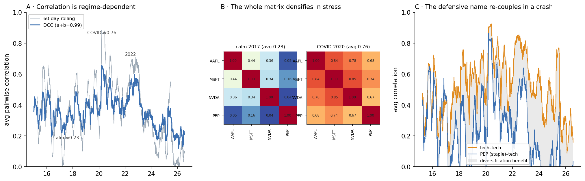
The DCC series (left panel) is not flat. Average pairwise correlation among the four stocks sits near 0.23 in the calm of 2017, then more than triples to ~0.76 in the COVID crash of March 2020, spikes again through 2022, and subsides afterwards. The calm-versus-crisis correlation matrices (middle panel) make it visceral: in 2017 the off-diagonal averages 0.23 and the staple PEP is almost uncorrelated with the tech names (0.05–0.16); in the 2020 crash the entire matrix reddens to an average of 0.76. This is the single most important fact about cross-asset dependence, and it is a risk fact, not a return fact: the diversification you measured in calm markets is not the diversification you have in a crisis, because the correlations that determine portfolio risk are themselves regime-dependent. A book sized on the long-run correlation is under-hedged exactly when a systemic move arrives.
4. The defensive asset re-couples — risk-on/off, made concrete
The clearest confirmation signal in this panel is the staple. PEP is a consumer-defensive name, and in normal times it genuinely diversifies a tech book: its average correlation to AAPL, MSFT and NVDA is 0.31, well below the 0.58 the tech names share with each other (the shaded gap in the right panel is that diversification benefit). But in the COVID crash the benefit evaporates — PEP’s correlation to tech jumps to 0.70 while tech-tech rises to 0.83. The defensive asset re-couples precisely in the crisis it was held to survive. This is risk-on/risk-off in miniature: in a risk-on regime, assets follow their own stories and cross-correlations are modest; in a risk-off regime, one systemic factor dominates and everything moves together. A specialist watching the spread between a defensive asset’s conditional correlation and its calm-market baseline has a direct, real-time read on which regime the market is in — exactly the “confirming vs contradicting” evidence the architecture asks this specialist to emit.
5. The factor and network views
The same fact wears two other hats. The factor view asks how much of the panel’s variance one common factor explains — the absorption ratio (Kritzman–Li), the share of total variance captured by the top principal components, \mathrm{AR}_k = \sum_{i=1}^{k}\lambda_i / \sum_{j=1}^{n}\lambda_j. A high, rising absorption ratio means the market is fragile — one factor is driving everything — which is the factor-model statement of “correlations went to one.” On this four-name panel the top component already explains ~0.73 of variance and rises only mildly in stress (~0.80→0.83), because four tech-heavy stocks share a dominant factor at all times; the measure earns its keep on a broad, multi-class panel (equities, rates, FX, credit, commodities), where the absorption ratio genuinely swings between diversified and systemic regimes. The network view (Gaussian graphical models) goes further, using the inverse covariance (precision) matrix \Theta=\Sigma^{-1} to read partial correlations — the direct links between assets after controlling for the rest — and watches the dependency network densify as a crisis spreads. All three are the same phenomenon seen through different lenses; DCC gives the time-varying pairwise picture, the absorption ratio compresses it to a systemic scalar, and the network exposes its structure.
6. What are its strengths?
- It measures the risk that actually bites. Portfolio risk is driven by conditional correlations, and DCC estimates them as they change — capturing the crisis concentration a static matrix hides.
- Valid correlation matrices, cheaply. The DCC rescaling guarantees a proper correlation matrix at every step from just two parameters, so it scales to many assets without exploding.
- A single systemic scalar. The absorption ratio compresses the whole dependence structure into one interpretable “how risk-off is the market” number a risk agent can act on.
- Directly a confirmation signal. The spread between a defensive asset’s conditional correlation and its calm baseline is a real-time risk-on/off read — precisely the cross-asset evidence the specialist exists to provide.
- Composable with regime tools. Dependence spikes coincide with regime transitions and change-points, so this layer reinforces the rest of the state estimate.
7. What are its weaknesses?
- All-equity panels understate it. Demonstrated here on four tech-ish stocks, the baseline correlation is high and the factor structure is always concentrated; the risk-on/off swing is far sharper on a genuine multi-class panel, which is the specialist’s real input.
- DCC is a scalar-dynamics simplification. One pair (a,b) governs all correlations, so every pair moves on the same clock — realistic enough for a signal, too coarse for fine structure (block or asymmetric DCC relax it).
- Correlation is not causation or direction. A dependence spike says assets are moving together, not why or which way — it is a risk and confirmation signal, never a return forecast.
- Estimation noise in the tails. Correlations are hardest to estimate exactly when they matter most — in fast crises with few observations — so the crisis reading is the noisiest one.
- Gaussian dependence misses tail co-movement. Linear correlation understates the joint-crash behaviour that copulas capture; assets can be modestly correlated in the body and near-perfectly correlated in the left tail.
8. How could it apply to markets?
This is the proposal’s Cross-Asset Confirmation specialist, and the finding defines its job. Its output is not a price view but a dependence state: a conditional-correlation estimate (DCC), a systemic-concentration scalar (absorption ratio), and a confirming/contradicting verdict built from whether cross-asset moves are aligned. That verdict is what distinguishes, in the site’s worked example, an “ordinary technical pullback” from a “macro-driven risk-off transition” — the pullback has equities falling while rates, credit and the dollar do their own thing; the transition has them all moving together, which is a correlation spike this specialist would flag in real time. It feeds the risk layer directly: rising conditional correlation means falling true diversification, so the hard risk limits should tighten exposure as dependence concentrates — the correlation caps in the risk governance are exactly this signal made binding. And it is the cleanest statement of why a multi-agent, multi-evidence architecture beats a single model: the information that the market has flipped to risk-off is not in any one asset’s price, it is in the relationship between them — a quantity only a cross-asset view can see.
9. What does the Python code look like?
import numpy as np
from arch import arch_model
from scipy.optimize import minimize

# 1) de-volatilize each column with univariate GARCH -> standardized residuals Z (T x n)
Z = np.column_stack([arch_model(100*R[:, j], vol="GARCH", p=1, q=1)
                     .fit(disp="off").std_resid for j in range(R.shape[1])])
Qbar = np.cov(Z.T)

# 2) DCC(1,1): fit (a, b) by quasi-max-likelihood on the correlation part
def dcc_nll(p):
    a, b = p
    if a <= 0 or b <= 0 or a + b >= 0.9995: return 1e12
    Q, ll = Qbar.copy(), 0.0
    for t in range(len(Z)):
        if t: Q = (1-a-b)*Qbar + a*np.outer(Z[t-1], Z[t-1]) + b*Q
        d = 1/np.sqrt(np.diag(Q)); Rt = Q * np.outer(d, d)     # valid correlation matrix
        _, logdet = np.linalg.slogdet(Rt)
        ll += logdet + Z[t] @ np.linalg.solve(Rt, Z[t])
    return 0.5*ll

a, b = minimize(dcc_nll, [0.02, 0.95], method="Nelder-Mead").x   # -> 0.017, 0.970

# absorption ratio: share of variance in the top-k principal components (rolling)
def absorption(cov, k=1):
    ev = np.sort(np.linalg.eigvalsh(cov))[::-1]
    return ev[:k].sum() / ev.sum()
The DCC recursion is one line inside the loop; the rescaling to a valid correlation matrix is the trick that makes it work for many assets at once.
10. How would I explain it to a supervisor?
“The cross-asset specialist’s whole job is to say whether the market is risk-on or risk-off, and that lives in the dependence structure, which isn’t constant. I built a dynamic conditional correlation model from scratch — GARCH to strip each asset’s own volatility, then a GARCH-like recursion on the correlations, fit by maximum likelihood — and got a+b of 0.99, so correlations are persistent but do move. The headline is a risk fact: average pairwise correlation among four stocks went from about 0.23 in calm 2017 to 0.76 in the COVID crash, so it more than tripled — diversification fails exactly when you need it. The cleanest illustration is the consumer staple, PEP: it diversifies a tech book in normal times, correlation 0.31 versus 0.58 tech-to-tech, but in the crash it re-couples to 0.70. That spread — a defensive asset’s conditional correlation versus its calm baseline — is a direct real-time risk-on/off signal. There’s a factor version, the absorption ratio, the share of variance in the top principal component, which is a single ‘how systemic is the market’ number, and a network version using partial correlations. I’m honest that my panel is all equities, so the baseline correlation is high and the swing is muted; on a real cross-asset panel with rates, FX and credit the risk-off signal is much sharper. For my proposal this is what separates a technical pullback from a macro risk-off transition — the information isn’t in any one price, it’s in the relationships — and it’s the signal that should tighten the risk limits as correlation concentrates.”
Data: daily log returns of AAPL, MSFT, NVDA, PEP, 2015–2026 (2,903 obs). DCC(1,1) implemented from scratch — univariate GARCH(1,1) de-volatilization (via arch) then DCC quasi-MLE on standardized residuals: a = 0.0170, b = 0.9703, a + b = 0.9873. Average pairwise correlation: full sample 0.36; 60-day rolling mean ≈ 0.26 in 2017, 0.64 in 2020, 0.59 in 2022; static matrices 0.23 (calm 2017) vs 0.76 (COVID 2020). Absorption ratio (top-1 of 4 PCs, rolling 120-day): 0.73 full, 0.80 in 2017, 0.82 in 2020, 0.83 in 2022 — weakly discriminating on a small tech panel, noted as a limitation. Staple decoupling: PEP–tech average correlation 0.31 (full) / 0.70 (2020) vs tech–tech 0.58 (full) / 0.83 (2020). Every number was checked.