Do Hard Risk Limits Earn Their Keep, or Just Hold Less?
Re-testing H8 against a benchmark that carries the same risk — because every limit in the original also cut exposure
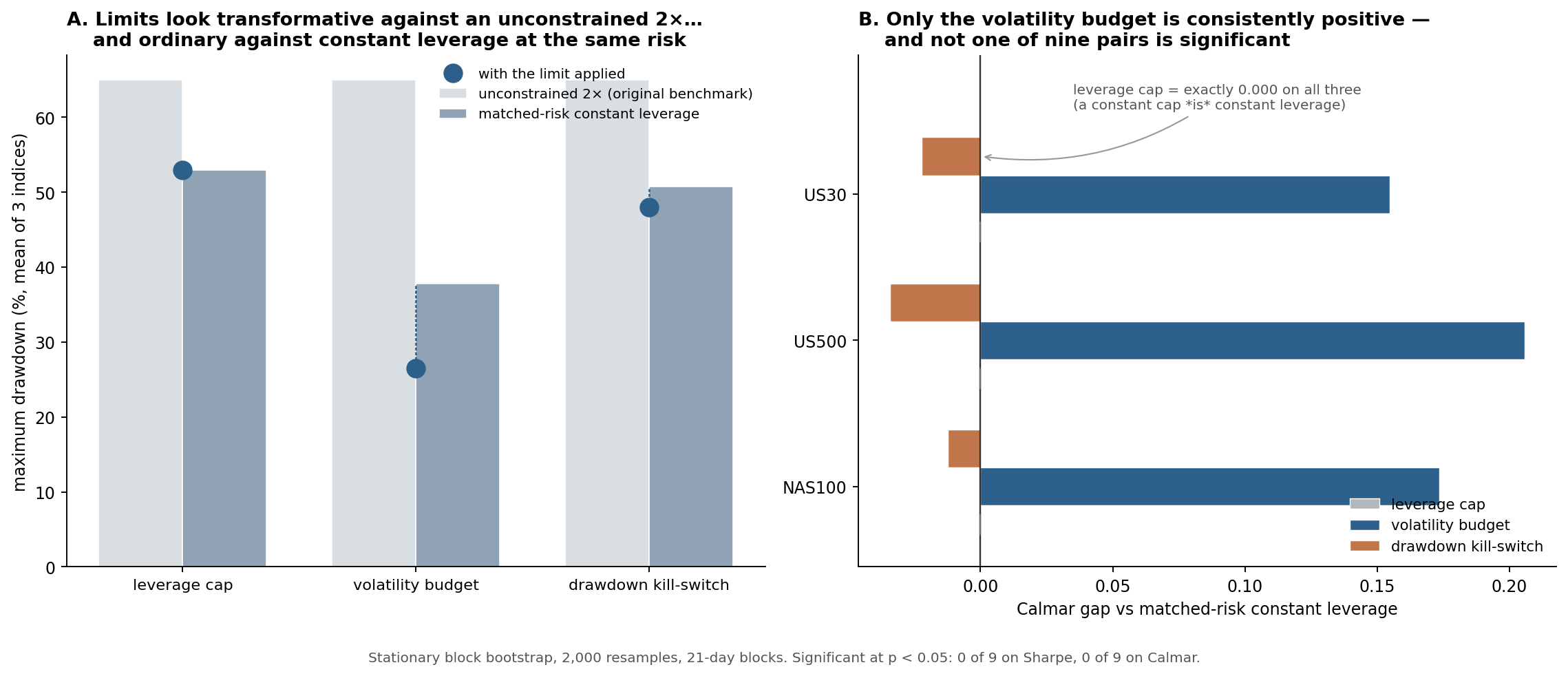
H8 says deterministic risk controls improve robustness and viability even where they cut return. The original tested a leveraged strategy with limits against the same strategy without them — but every limit reduces exposure, so drawdown falls for free and Calmar rises from reduced volatility drag. Re-tested against a constant leverage carrying the same realised volatility: the leverage cap does exactly nothing, the kill-switch is consistently worse, and the volatility budget is consistently better on all three assets without reaching significance in any of nine comparisons.
Why re-test this one
By the time RQ1, RQ2/H1 and H2 had been through the full protocol, only two of the proposal’s hypotheses had never faced it. H8 was the one I expected to survive: it is a claim about constraints rather than forecasts, and constraints are closer to arithmetic than to signal.
That expectation turned out to be right in an unhelpful way. The parts that are arithmetic are arithmetic all the way down — including the part the original counted as evidence.
The confound
The original experiment took a deliberately aggressive 2× leveraged long and layered hard limits on it: a leverage cap at 1.5×, a volatility/CVaR budget, and a drawdown kill-switch. The limited versions had far shallower drawdowns and better Calmar, and the conclusion was that hard limits turn an untradeable strategy into a viable one.
Every one of those limits also reduces exposure. A cap takes 2× to 1.5×. A volatility budget scales down. A kill-switch halves. So two effects are tangled together:
Drawdown falls because you hold less. This is the same artefact caught in the RQ1 overlay: a rule that cuts exposure always shows a shallower drawdown, whether or not it cuts it at useful moments.
Calmar is not scale-invariant. Under compounding, leverage k earns roughly k\mu - k^2\sigma^2/2 in log terms. Less leverage means less volatility drag, so a lower- leverage strategy tends to a better CAGR-to-drawdown ratio mechanically. “Capped beats uncapped on Calmar” is close to a statement about compounding rather than about risk management.
The benchmark that fixes it
Compare each limited strategy against a constant leverage scaled to carry the same realised volatility. Constant exposure has no risk management in it whatsoever — no cap, no budget, no reaction to anything. If a limit is worth having, it has to beat that.
Three indices — NAS100, US500, US30 — daily from 2015, net of 2bp on turnover, with the benchmark charged the same entry cost so a one-day fee cannot masquerade as underperformance. Significance by stationary block bootstrap (2,000 resamples, 21-day blocks), because daily returns are serially dependent in volatility and an i.i.d. bootstrap would manufacture significance for the same reason the forecasting tests need Newey-West.
Both Sharpe and Calmar are tested. That matters: Sharpe is a mean-variance measure and cannot see a rule that reshapes the tail without changing mean-variance efficiency — which is precisely what a drawdown control is supposed to do.
Results
The leverage cap does exactly nothing — and that is not a figure of speech.
| Sharpe gap | Calmar gap | p | |
|---|---|---|---|
| NAS100 | −0.000 | 0.000 | 1.00 |
| US500 | 0.000 | 0.000 | 1.00 |
| US30 | −0.000 | −0.000 | 1.00 |
A constant leverage cap is constant leverage. Once the benchmark is constant leverage at the same volatility, the two strategies are the same strategy and there is nothing left to measure. The entire apparent benefit in the original is the arithmetic of holding less.
Finding that required fixing a bug in my own test: when two return streams are identical the bootstrap has zero variance, and floating-point noise was reading as p = 0.010. The test now detects the degenerate case and reports p = 1.00.
The kill-switch is consistently worse. Sharpe gaps of −0.068, −0.069 and −0.057; Calmar negative on all three. Directionally this confirms the original’s own finding that reactive drawdown rules backfire — selling after the fall and buying back after the recovery.
The volatility budget is the one that might be real. It is positive on all three assets on both metrics — six for six in sign:
| Sharpe gap | Calmar gap | p (Calmar) | |
|---|---|---|---|
| NAS100 | +0.099 | +0.173 | 0.26 |
| US500 | +0.060 | +0.206 | 0.19 |
| US30 | +0.051 | +0.155 | 0.29 |
The Calmar gains are large in relative terms — a mean of +0.178 against a matched-risk Calmar of roughly 0.30, so about +60%. And the pattern is exactly what a risk control should look like: a big improvement in drawdown-per-unit-of-return with only a small change in Sharpe, meaning it is reshaping the tail rather than improving mean-variance efficiency.
But nothing is significant. Zero of nine comparisons on Sharpe, zero of nine on Calmar.
The verdict — H8 does not survive, with one live thread
H8 as stated is not supported. Against a benchmark carrying the same risk, hard limits do not demonstrably improve viability. One of the three does nothing at all by construction, one is consistently harmful, and the third is consistently helpful but never distinguishable from noise on three correlated indices.
The volatility budget deserves a proper test rather than a verdict. Six-for-six in sign with a ~60% relative Calmar gain is the most promising unfalsified result anywhere in this lab. It is also exactly the signature that has repeatedly failed to survive widening — ewma_slope was 7 for 7 in sign and cleared the bar on 2 of 7 assets; the H2 residual was 3 for 3 and cleared nothing. Consistent-but-never-significant has been this lab’s most reliable false positive.
This completes the audit, and the result is uncomfortable. Every hypothesis that has now faced the full protocol — RQ1, RQ2/H1, H5, H2 and H8 — has returned a null or a near-null. Only H6 (benefit concentrating at transitions) remains untested. The proposal’s empirical position is that its architecture is not yet supported by its own evidence, and the honest thing is to say so rather than to keep the earlier verdicts on the page.
Limitations
- Not an exact replication. The original used a 2016 out-of-sample start and different budget parameters; this uses 2015 and the harness’s own settings, so the absolute drawdowns differ from the published −63% → −26%. It tests the same claim under a fair benchmark, not the same code.
- Three correlated indices. Nine comparisons are nowhere near nine independent tests. With a deflated bar this would be harder still, so “0 of 9” is already generous.
- One matched-risk definition. Matching on realised volatility is the natural choice, but matching on average exposure or on ex-ante volatility would give slightly different benchmarks.
- The volatility budget is under-powered here, not disproven. Three assets cannot resolve a Calmar gap of this size at p < 0.05. A seven-asset test is the obvious next step and the one I would run before drawing any conclusion about it.
- Costs are simple. 2bp on turnover, no slippage model, no financing cost on leverage — and financing would hurt the higher-exposure strategies most, so the comparison is if anything generous to the unconstrained base.
What I learned
A constraint that is a constant is not a constraint. The leverage cap result is the cleanest thing in this entry: comparing “2× capped at 1.5×” against “2× uncapped” tells you about 1.5× versus 2×, which you already knew. The only informative comparison is against something carrying the same risk, and once you build it the cap has nothing to say.
The wider lesson is the one this lab has now learned four separate ways: the benchmark is where the result lives. Raw drawdown versus an unconstrained base, a tercile rule versus a filtered HMM, own-span scoring versus a common window, a rich model versus a small one — each time the treatment was fine and the comparison was doing the work. Effect sizes get scrutinised. Benchmarks mostly do not.
NAS100, US500, US30 daily from 2015 (--offline, committed CSVs). Base strategy: 2× leveraged long, net 2bp on turnover. Limits: leverage cap 1.5×; volatility budget ≈17.5% annualised via min(2, budget/rv20); drawdown kill-switch halving exposure after a −20% trailing drawdown. Benchmark: constant leverage m set so realised volatility matches the limited strategy’s, charged the same day-one entry cost. Significance: stationary block bootstrap, 2,000 resamples, 21-day blocks, on both Sharpe and Calmar differences, with a degeneracy guard for the case where the two return streams coincide. Results: leverage cap gap exactly 0.000 on all three assets (p = 1.00); kill-switch Sharpe −0.068 / −0.069 / −0.057; volatility budget Sharpe +0.099 / +0.060 / +0.051 and Calmar +0.173 / +0.206 / +0.155 (p = 0.26 / 0.19 / 0.29). Significant at p < 0.05: 0 of 9 on Sharpe, 0 of 9 on Calmar. Code in src/msl/metrics/risklimits.py of the market-state-lab harness.